35 Data Visualization - Other

In section, more graphical parameters, including annotations, axes, themes and legends, will be illustrated.

Again, let us first load the tidyverse package.

library(tidyverse)

35.1 Annotations

Displaying just your data usually isn’t enough – there’s all sorts of other information that can help the viewer interpret the data. In addition to the standard repertoire of axis labels, tick marks, and legends, you can also add individual graphical or text elements to your plot. These elements can be used to add extra contextual information, highlight an area of the plot, or add some descriptive text about the data.

35.1.1 Adding text annotations

This can be done using annotate() and a text geom.

ggplot(iris, aes(Petal.Width, Petal.Length, color = Species)) +
  geom_point() +
  annotate("text", x = 0.25, y = 2.25, label = "setosa") +
  annotate("text", x = 1.25, y = 2.5, label = "versicolor") +
  annotate("text", x = 2.2, y = 4.5, label = "virginica")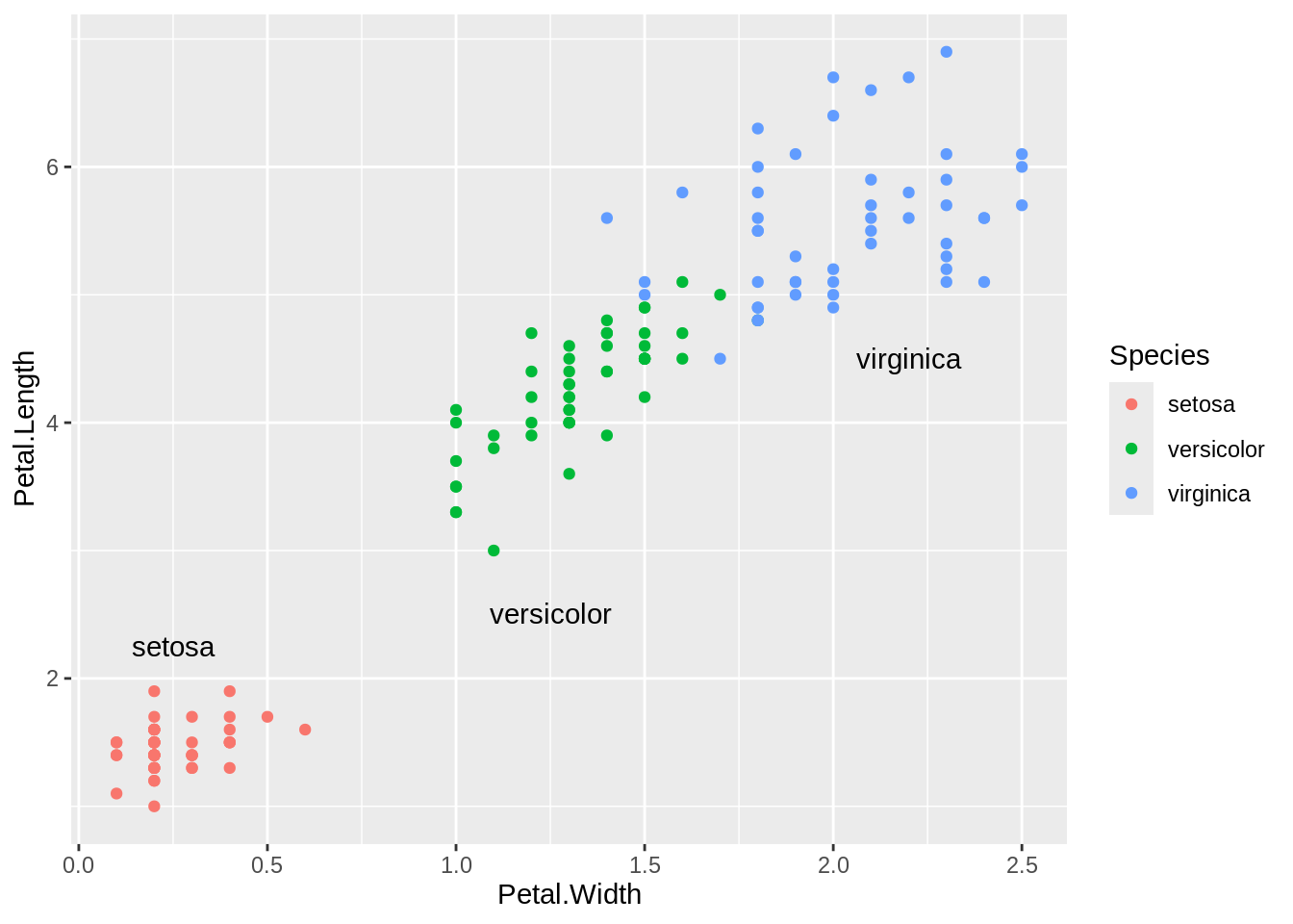

The annotate() function can actually be used to add any type of geometric object. In this case, we used geom = "text". Other text properties can be specified. The variables are mostly self-explanatory:

ggplot(iris, aes(Petal.Width, Petal.Length, color = Species)) +
  geom_point() +
  annotate("text", x = 0.25, y = 2.25, label = "setosa", 
           family = "serif", fontface = "italic", 
           color = "darkred", size = 3) +
  annotate("text", x = 1.25, y = 2.5, label = "versicolor",
           family = "serif", fontface = "italic", 
           color = "darkred", size = 3) +
  annotate("text", x = 2.2, y = 4.5, label = "virginica",
           family = "serif", fontface = "italic", 
           color = "darkred", size = 3)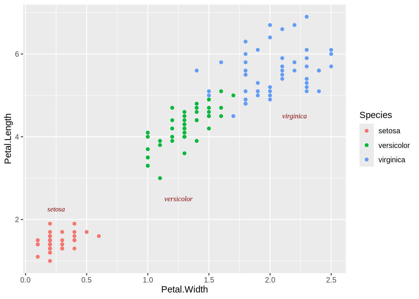

If the axes are continuous, you can use the special values Inf and -Inf to place text annotations at the edge of the plotting area. You will also need to adjust the position of the text relative to the corner using hjust and vjust - if you leave them at their default values, the text will be centered on the edge. It may take a little experimentation with these values to get the text positioned to your liking:

ggplot(iris, aes(Petal.Width, Petal.Length)) +
  geom_point() +
  annotate("text", x = -Inf, y = Inf, label = "Upper left", 
           hjust = -0.2, vjust = 2) +
  annotate("text", x = mean(range(iris$Petal.Width)), 
           y = -Inf, vjust = -0.4,
           label = "Bottom middle")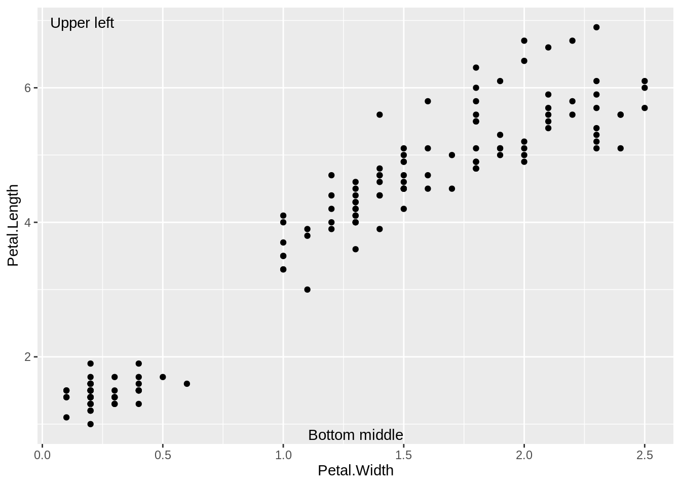

We can also add a text annotation with mathematical notation. Again, we use annotate(geom = "text"), but with parse = TRUE.

# A normal curve
ggplot(data.frame(x = c(-3, 3)), aes(x = x)) +
  stat_function(fun = dnorm) +
  annotate("text", x = 2, y = 0.3, parse = TRUE,
           label = "frac(1, sqrt(2 * pi)) * e ^ {-x^2 / 2}")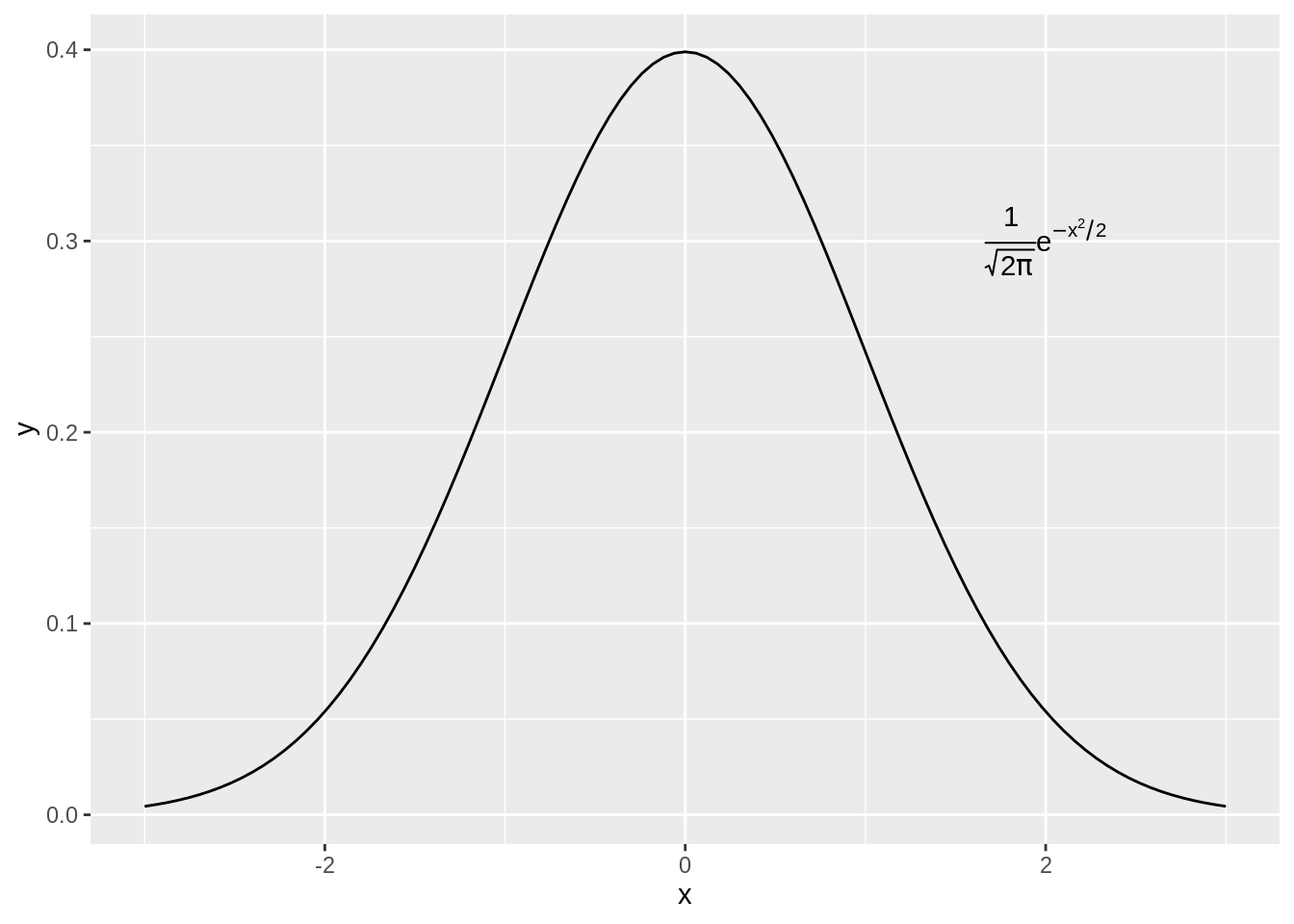

See ?plotmath for many examples of mathematical expressions, and demo(plotmath) for graphical examples of mathematical expressions.

Exercise A

Draw boxplots of weight grouped by different experiment group.

Indicate the outliers using an annotation with the text “outliers” where appropriate. Set the font to italic and the color to “orange”.

35.1.2 Adding lines

We can easily add horizontal and vertical lines using geom_hline() and geom_vline(), and angled lines, using geom_abline().

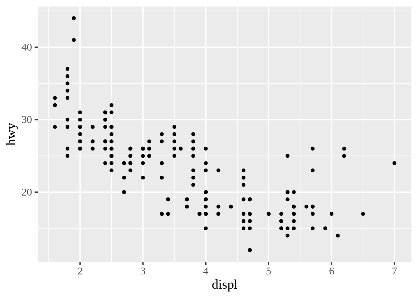
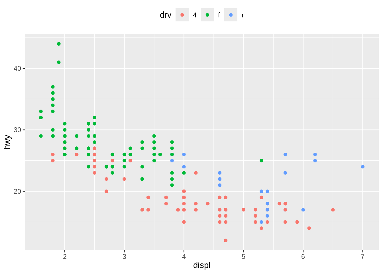
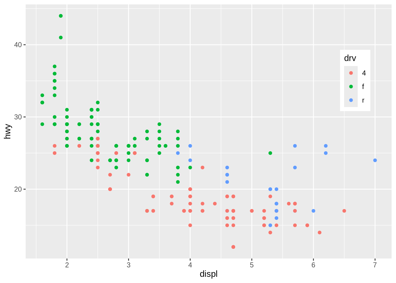
fueleco_plot <- ggplot(mpg, aes(displ, hwy, color = drv)) +
  geom_point()

# Add horizontal and vertical lines
fueleco_plot +
  geom_hline(yintercept = 30) +
  geom_vline(xintercept = 4.5)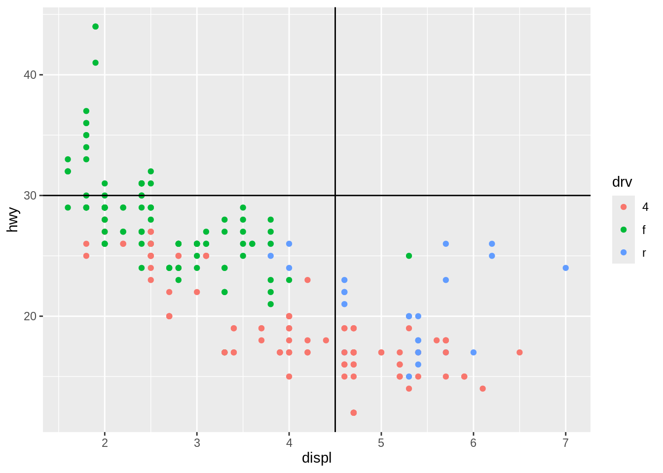

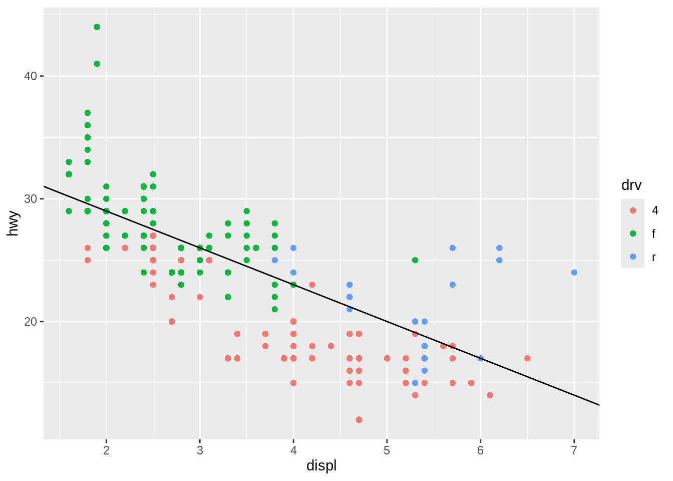
# Add angled line
fueleco_plot +
  geom_abline(intercept = 35, slope = -3)

The previous examples demonstrate setting the positions of the lines manually, resulting in one line drawn for each geom added. It is also possible to map values from the data to xintercept, yintercept, and so on, and even draw them from another data frame.

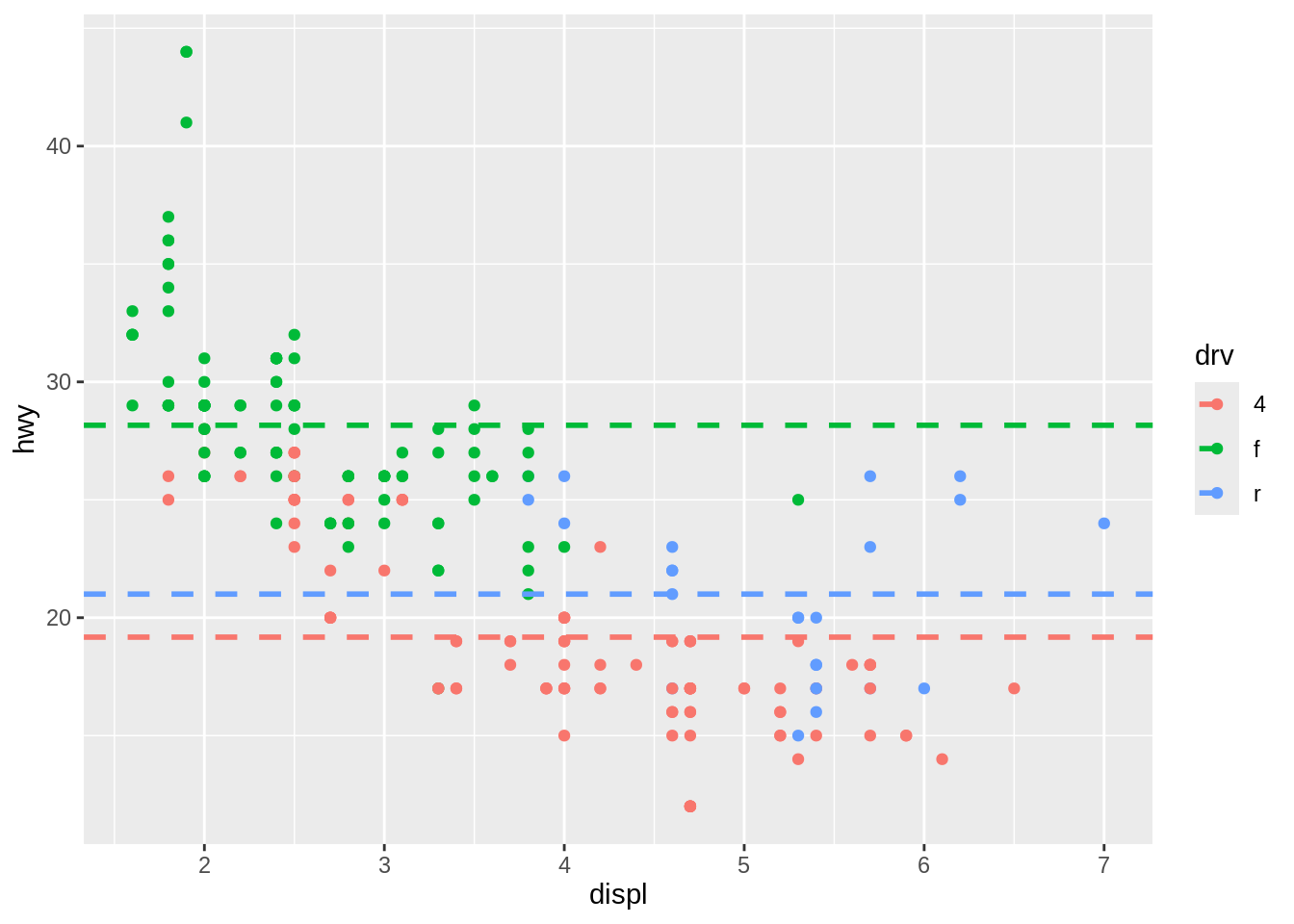
Here we’ll take the average hwy for different drive trains and store it in a data frame, hwy_means.

hwy_means <- mpg %>% 
  group_by(drv) %>% 
  summarise(meanhwy = mean(hwy))
hwy_means

Then we’ll draw a horizontal line for each, and set the linetype and linewidth.

fueleco_plot + 
  geom_hline(
    data = hwy_means,
    aes(yintercept = meanhwy, color = drv),
    linetype = "dashed",
    linewidth = 1
  )

If one of the axes is discrete rather than continuous, you can specify the intercepts either as a character string or as numbers. If the axis represents a factor, the first level has a numeric value of 1, the second level has a value of 2, and so on. You can specify the numerical intercept manually, or calculate the numerical value using which(levels(...)).

irislen_plot <- ggplot(iris, aes(Species, Petal.Length)) +
  geom_point()

# Add a vertical line for versicolor
irislen_plot +
  geom_vline(xintercept = 2)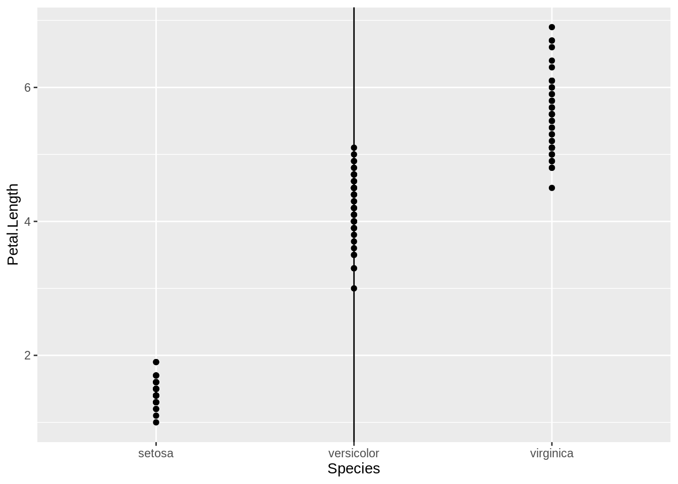

# Add a vertical line for setosa
irislen_plot +
  geom_vline(xintercept = 
               which(levels(iris$Species) == "setosa"))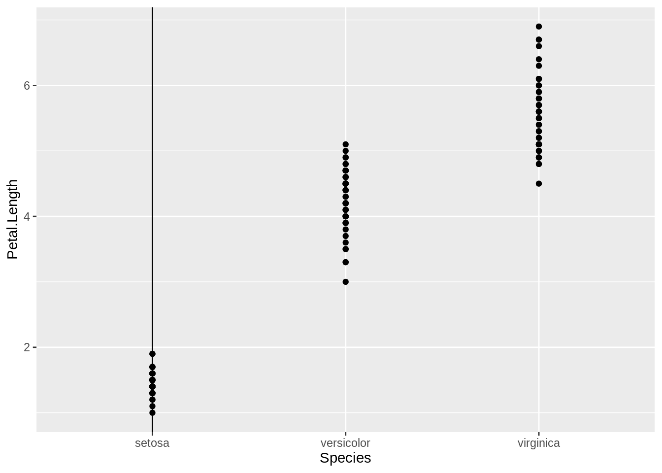

Exercise B

Work with the PlantGrowth data set.

Create histograms of weight for different experiment group.

Use appropriate binwidths and different bin colors for different experiment group.
You should also set the transparency of the bins to 0.5.

Add vertical lines to the histograms.

Each vertical line should represent the mean value of weight for each experiment group.
Color the vertical lines according to experiment group.
All vertical lines should be “dotdash”.
Set the width of the lines to 0.8.

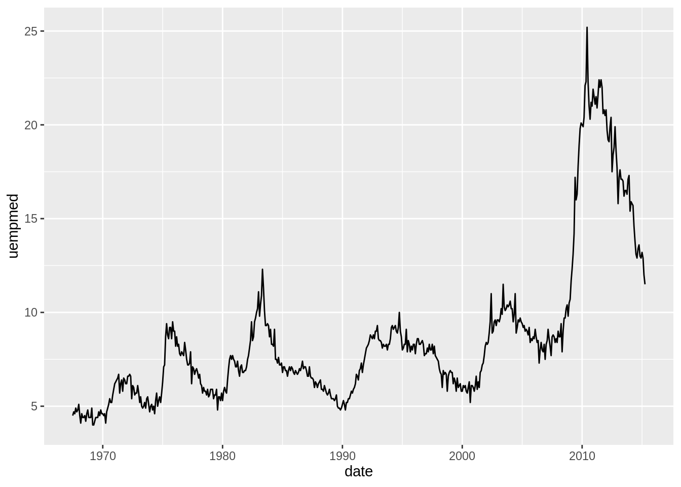
We can also add segmented lines using annotate("segment"). In this example, let us work with the economics data for illustration. We can initially generate a line plot for median unemployment duration (in weeks) overtime.

unemp_plot <- ggplot(economics, aes(date, uempmed)) + 
  geom_line()
unemp_plot

Then, let us highlight the period from 1980 to 1990 using a segmented line.

unemp_plot + 
  annotate("segment", x = as.Date("1980-01-01", "%Y-%m-%d"), 
           xend = as.Date("1990-01-01", "%Y-%m-%d"), 
           y = 15, yend = 15)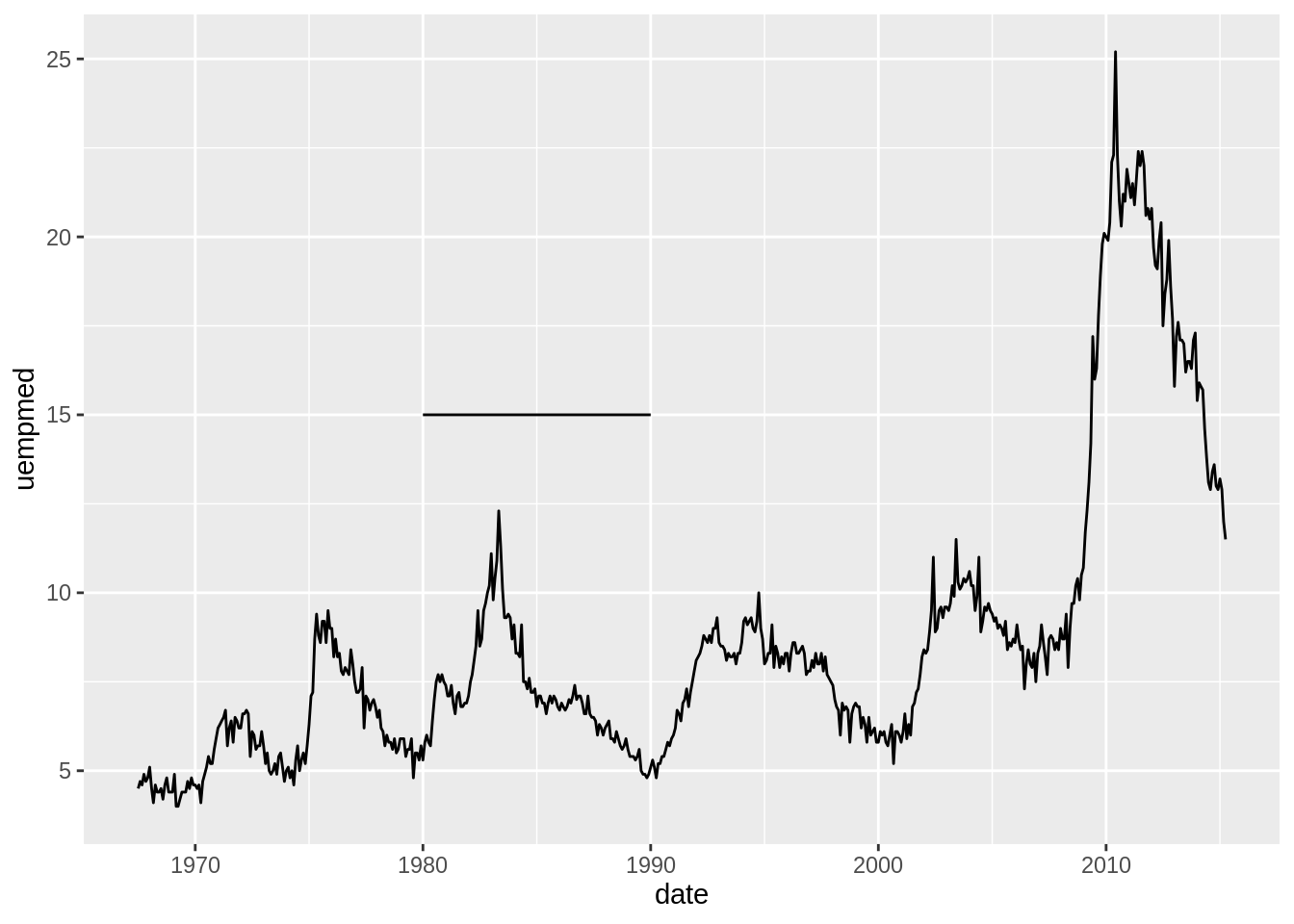

It’s possible to add arrowheads or flat ends to the line segments, using arrow(). In this example, we’ll do both.

unemp_plot + 
  annotate("segment", 
           x = as.Date("2000-01-01", "%Y-%m-%d"), 
           xend = as.Date("2010-01-01", "%Y-%m-%d"), 
           y = 10, yend = 25,
           linewidth = 2, color = "pink", arrow = arrow()) +
  annotate("segment", 
           x = as.Date("1980-01-01", "%Y-%m-%d"), 
           xend = as.Date("1990-01-01", "%Y-%m-%d"), 
           y = 15, yend = 15,
           arrow = arrow(ends = "both", angle = 90, 
                         length = unit(0.2, "cm")))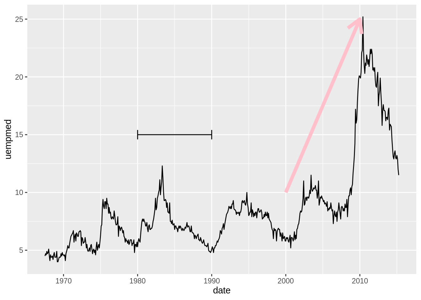

The default angle is 30, and the default length of the arrowhead lines is 0.2 inches.

If one or both axes are discrete, the \(x\) and \(y\) positions are such that the categorical items have coordinate values 1, 2, 3, and so on.

Exercise C

Work with the PlantGrowth data set.

Draw a boxplot demonstrating the overall distribution of weight.

Annotate with a line segment representing the mean value of weight. You may need to adjust the starting and ending points of the \(x\)-axis multiple times to find the most suitable positions.

Color the line segment from 2. in “purple”.

35.1.3 Adding a shaded rectangle

annotate("rect") will allow us to add rectangles on our plot.

unemp_plot + 
  annotate("rect", 
           xmin = as.Date("1980-01-01", "%Y-%m-%d"),
           xmax = as.Date("1990-01-01", "%Y-%m-%d"),
           ymin = 1, ymax = 25,
           alpha = 0.1, fill = "red")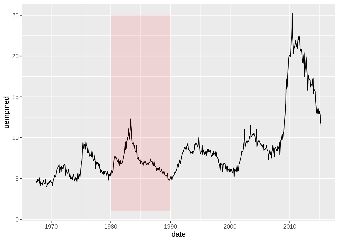

Each layer is drawn in the order that it’s added to the ggplot object, so in the preceding example, the rectangle is drawn on top of the line. It’s not a problem in that case, but if you’d like to have the line above the rectangle, add the rectangle first, and then the line.

Any geom can be used with annotate(), as long as you pass in the proper parameters. In this case, geom_rect() requires min and max values for \(x\) and \(y\).

35.1.4 Adding error bars

Sometimes we would like to add error bars to a graph. That can be done by geom_errorbar() and map variables to the values for ymin and ymax.

Let us first calculate means and standard errors and save them in a data frame.

hwy_summary <- mpg %>% 
  group_by(drv) %>% 
  summarise(n = n(), meanhwy = mean(hwy), sdhwy = sd(hwy)) %>% 
  mutate(se = sdhwy / sqrt(n))
hwy_summary

Adding the error bars is done the same way for bar graphs and line graphs.

# bar plot
ggplot(hwy_summary, aes(drv, meanhwy)) + 
  geom_col() +
  geom_errorbar(aes(ymin = meanhwy - se, 
                    ymax = meanhwy + se), 
                width = 0.2)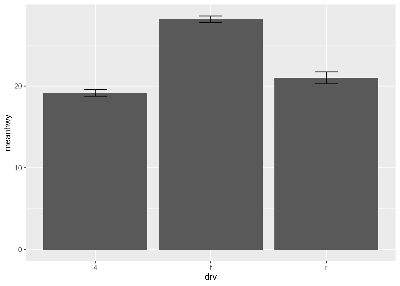

# line plot
ggplot(hwy_summary, aes(drv, meanhwy)) + 
  geom_line(aes(group = 1)) +
  geom_point(size = 2) +
  geom_errorbar(aes(ymin = meanhwy - se, 
                    ymax = meanhwy + se), 
                width = 0.2)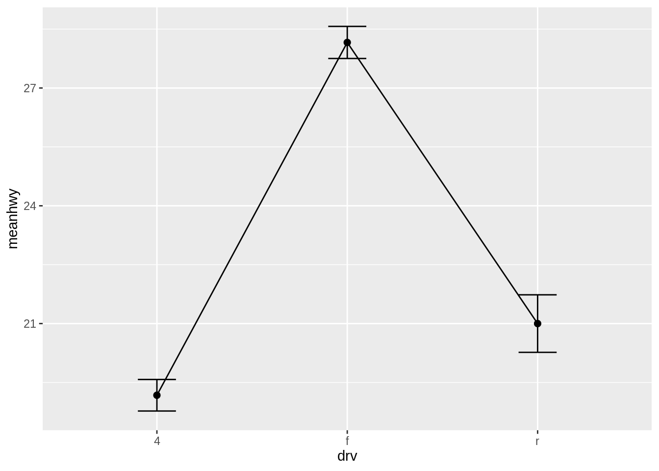

In this example, we calculated values for the standard error of the mean (se), which are used for the error bars (values for the standard deviation, sd, were also computed, but we’re not using that here).

To get the values for ymax and ymin, we took the \(y\) variable, meanhwy, and added/subtracted se.

We also specified the width of the ends of the error bars, with width = 0.2. It’s best to play around with this to find a value that looks good. If you don’t set the width, the error bars will be very wide, spanning all the space between items on the \(x\)-axis.

Exercise D

Work with the ToothGrowth data set.

First, create a data frame displaying aggregated information based on the supp variable. Each unique value of supp will be accompanied by the mean values of tooth lengths (len) and their corresponding standard errors of the means.

Create a barplot comparing the mean lengths across supplements, including error bars using standard errors.

35.2 Axes

35.2.1 Changing the order of items on a discrete axis

For a categorical (or discrete) axis - one with a factor mapped to it - the order of items can be changed by setting limits in scale_x_discrete() or scale_y_discrete().

Let us first convert the drv column into a factor type:

mpgexample <- mpg %>% mutate(drv = as.factor(drv))
class(mpgexample$drv)

[1] "factor"

levels(mpgexample$drv)

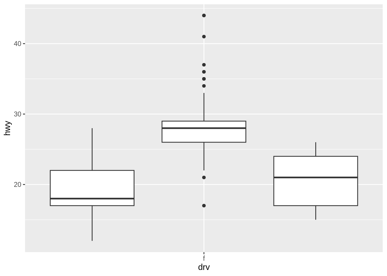
[1] "4" "f" "r"

To manually set the order of items on the axis, specify limits with a vector of the levels in the desired order. You can also omit items with this vector.

ggplot(mpgexample, aes(drv, hwy)) +
  geom_boxplot() +
  scale_x_discrete(
    limits = c("f", "4", "r"))

You can also use this method to display a subset of the items on the axis.

ggplot(mpgexample, aes(drv, hwy)) +
  geom_boxplot() +
  scale_x_discrete(
    limits = c("f", "r"))

Warning: Removed 103 rows containing missing values or values outside the scale range
(`stat_boxplot()`).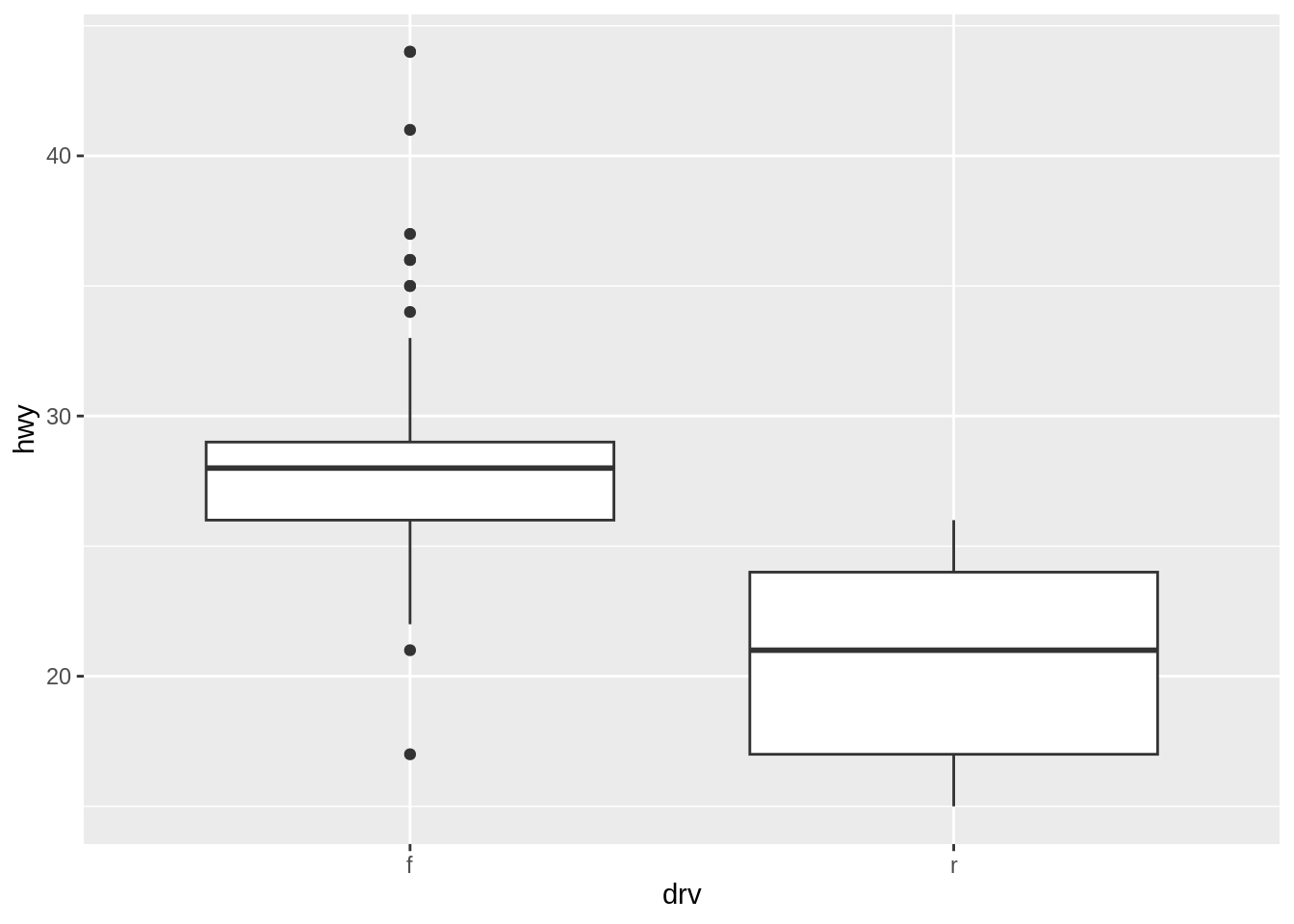

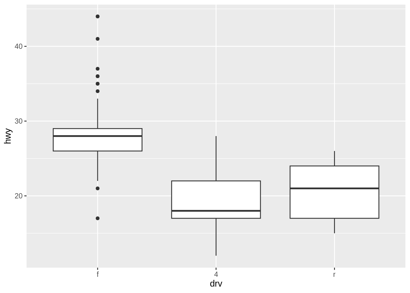
To reverse the order, set limits = rev(levels(...)), and put the factor inside.

ggplot(mpgexample, aes(drv, hwy)) +
  geom_boxplot() +
  scale_x_discrete(
    limits = rev(levels(mpgexample$drv)))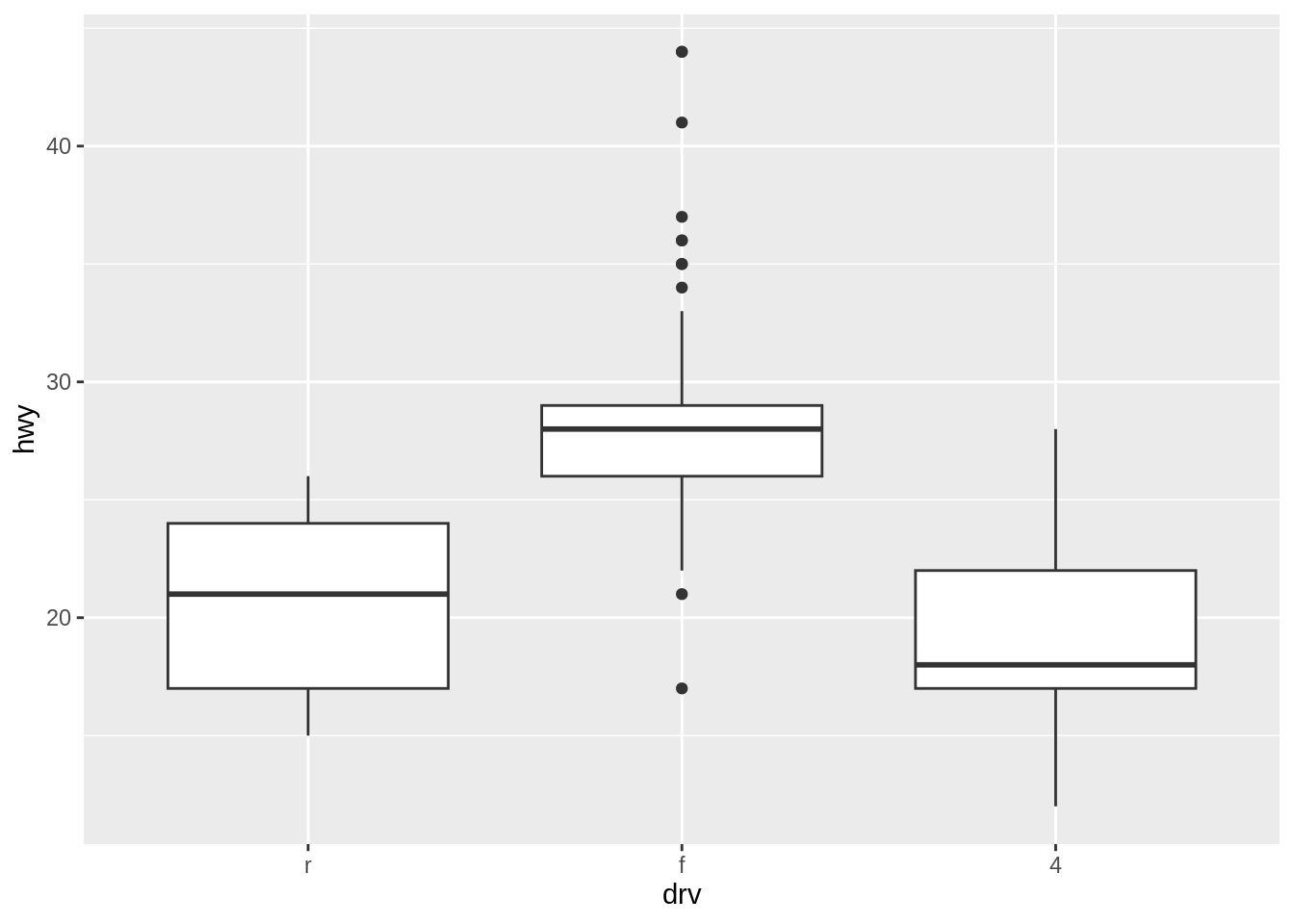

Exercise E

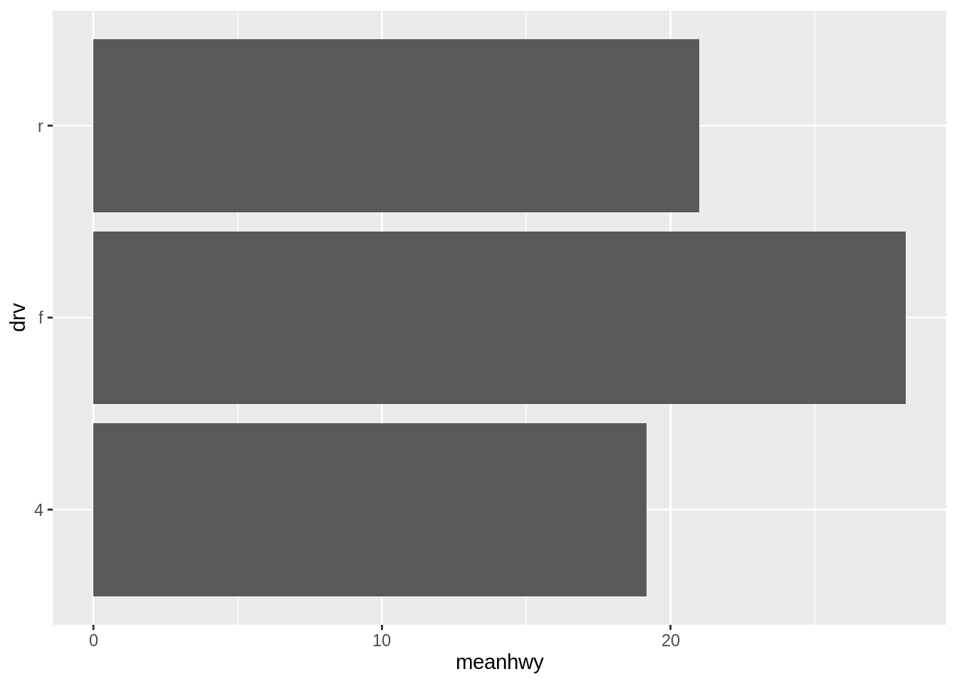
Analyze the PlantGrowth dataset. Create a boxplot of weight with the group arranged in the order of “trt1,” “trt2,” “ctrl.”

35.2.2 Swaping \(x\)- and \(y\)- axes

We can use coord_flip() to flip the axes.

ggplot(hwy_summary, aes(drv, meanhwy)) + 
  geom_col() +
  coord_flip()

Exercise F

Work with the PlantGrowth data set.

Create a bar chart of the mean weight values by experiment group. Remember to start by creating a data frame that contains the mean weight values grouped by their respective categories.

Reverse the coordinates, making the \(x\)-axis represent the mean values of weight and the \(y\)-axis represent group.

35.2.3 Setting the positions of tick marks

Usually ggplot does a good job of deciding where to put the tick marks, but if you want to change them, set breaks in the scale.

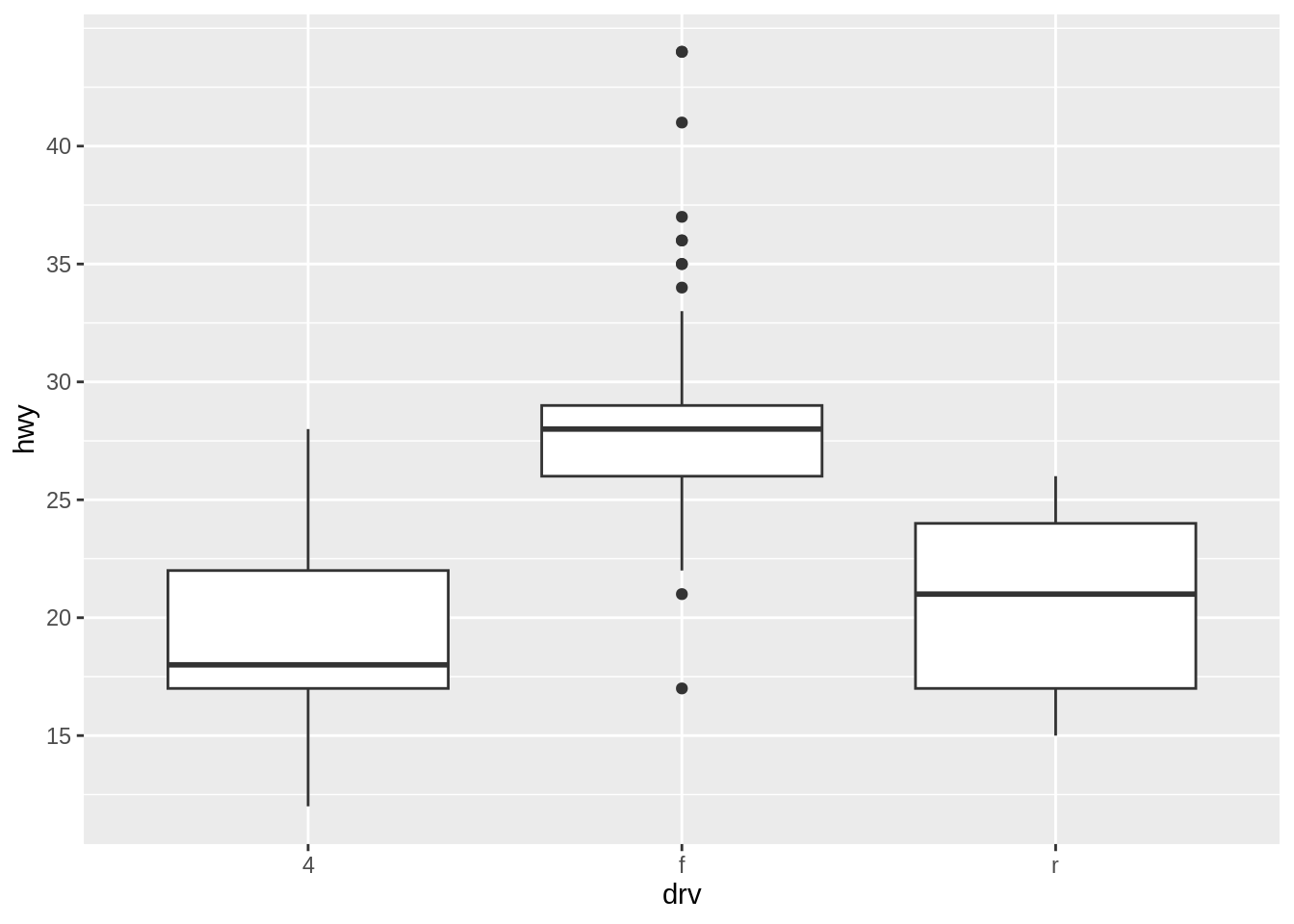
ggplot(mpg, aes(drv, hwy)) +
  geom_boxplot() +
  scale_y_continuous(
    breaks = c(10, 12, 16, 20, 25, 30, 40))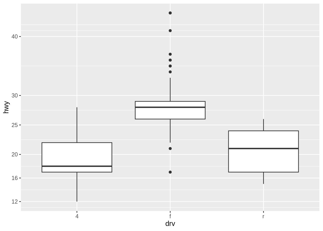

The location of the tick marks defines where major grid lines are drawn. If the axis represents a continuous variable, minor grid lines, which are fainter and unlabeled, will by default be drawn halfway between each major grid line.

You can also use the seq() function or the : operator to generate vectors for tick marks:

ggplot(mpg, aes(drv, hwy)) +
  geom_boxplot() +
  scale_y_continuous(
    breaks = seq(10, 40, by = 5))

If the axis is discrete instead of continuous, then there is by default a tick mark for each item. For discrete axes, you can change the order of items or remove them by specifying the limits, as mentioned before. Setting breaks will change which of the levels are labeled, but will not remove them or change their order. Below shows what happens when you set breaks.

ggplot(mpg, aes(drv, hwy)) +
  geom_boxplot() +
  scale_x_discrete(
    breaks = "f")

Exercise G

Work with the PlantGrowth data set.

Again, draw boxplots of weight by experiment group.

Adjust the y-axis ticks to have breaks at 4, 4.25, 4.5, 5, 6, and 8.

35.2.4 Changing the tick labels

To set arbitrary labels, pass values to breaks and labels in the scale. One of the labels has a newline \\n character, which tells ggplot to put a line break there:

hwy_plot <- ggplot(mpg, aes(displ, hwy)) + 
  geom_point()
hwy_plot + 
  scale_y_continuous(
    breaks = seq(15, 35, by = 5),
    labels = c("Really\nLow", "Low", 
               "Medium", "High", 
               "Really\nHigh"))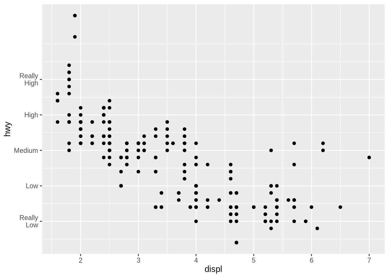

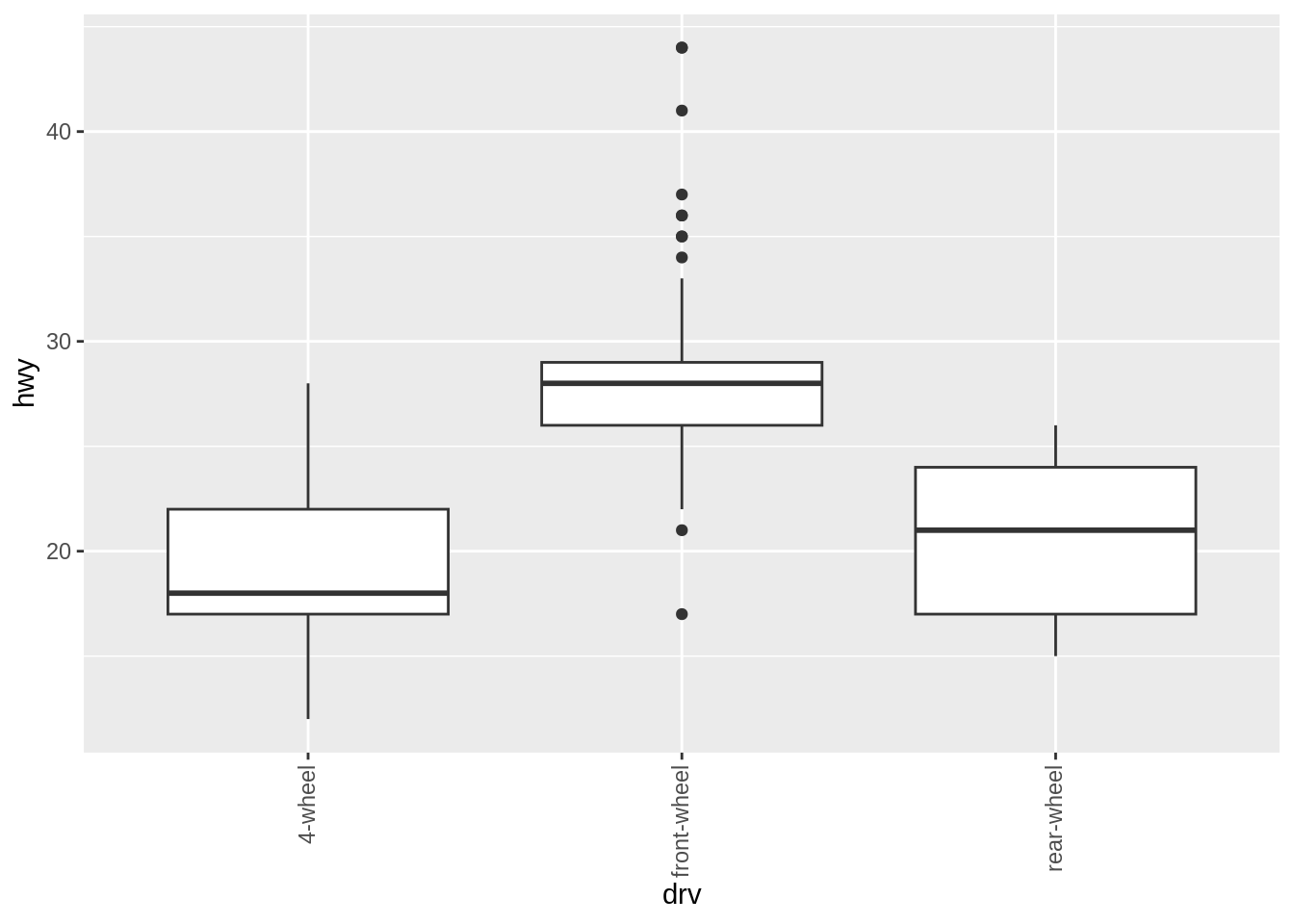
We could also modify the appearance of the tick labels. Let us first create the boxplots of hwy by drv.

hwy_boxplot <- ggplot(mpg, aes(drv, hwy)) +
  geom_boxplot() +
  scale_x_discrete(
    breaks = c("4", "f", "r"),
    labels = c("4-wheel",
               "front-wheel", 
               "rear-wheel"))
hwy_boxplot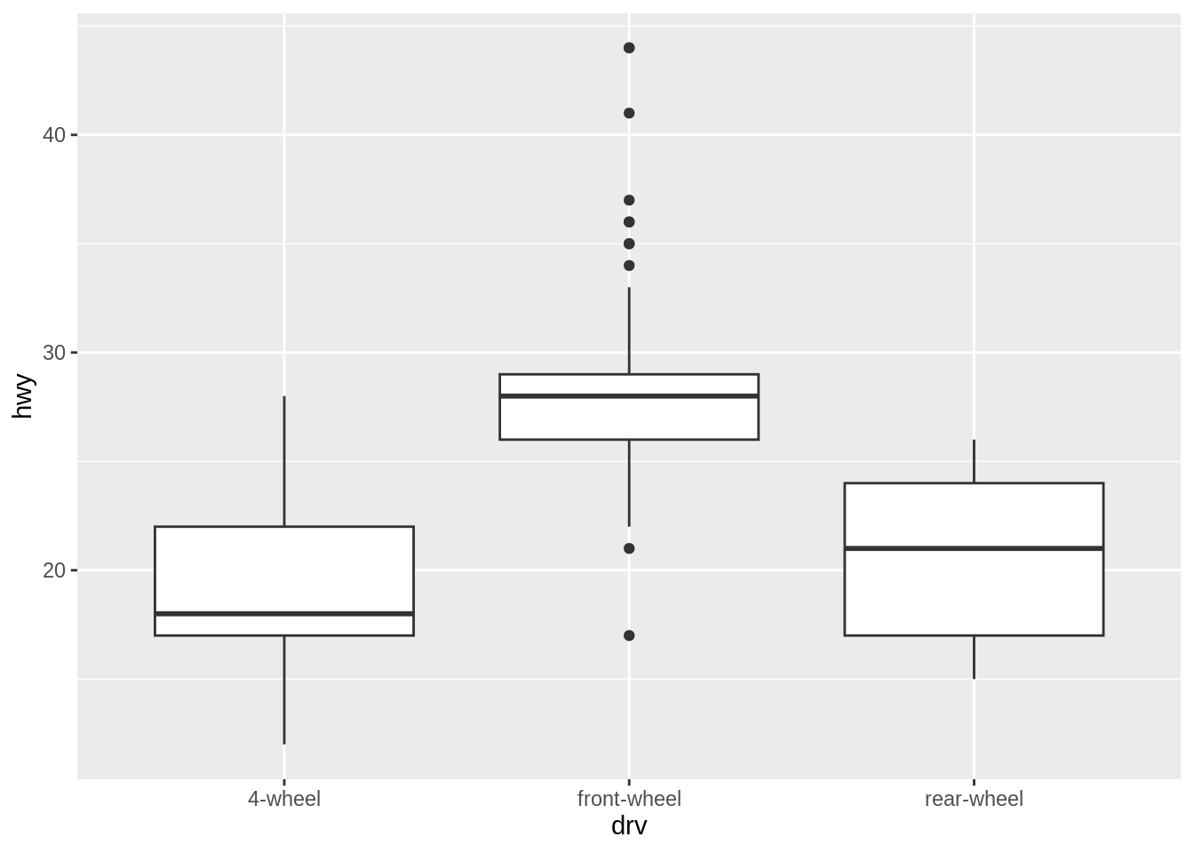

To rotate the text 90 degrees counterclockwise:

hwy_boxplot +
  theme(axis.text.x = 
          element_text(
            angle = 90, 
            hjust = 1, 
            vjust = 0.4))

Rotating the text 30 degrees uses less vertical space and makes the labels easier to read without tilting your head:

hwy_boxplot + 
  theme(axis.text.x = 
          element_text(
            angle = 30, 
            hjust = 0.5, 
            vjust = 1))

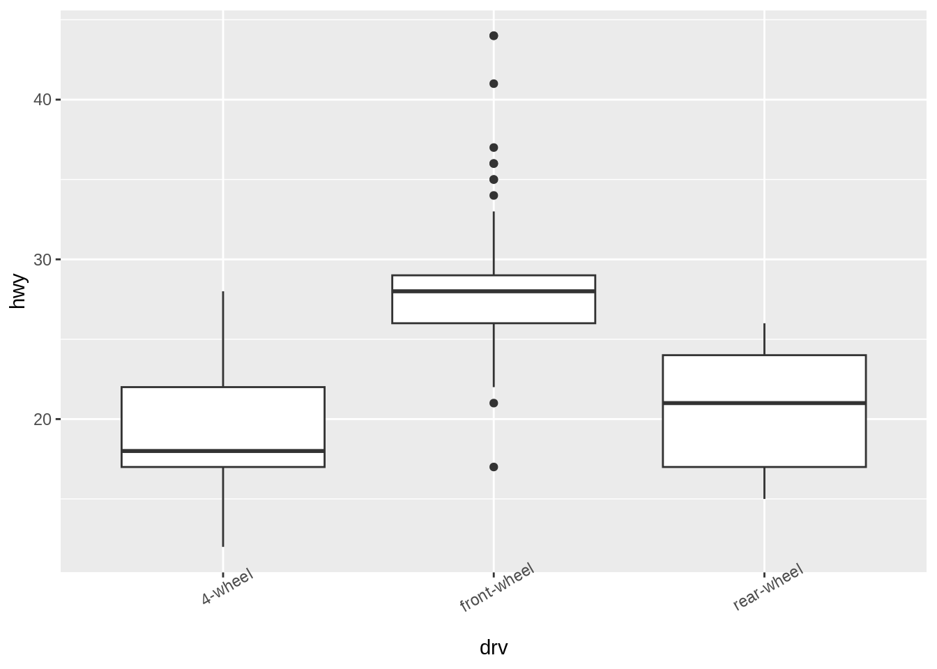
The hjust and vjust settings specify the horizontal alignment (left/center/right) and vertical alignment (top/middle/bottom).

Besides rotation, other text properties, such as size, style (bold/italic/normal), and the font family (such as Times or Helvetica) can be set with element_text().

hwy_boxplot +
  theme(axis.text.x = 
          element_text(
            family = "Times", 
            face = "italic",
            color = "darkred",
            size = rel(0.9)))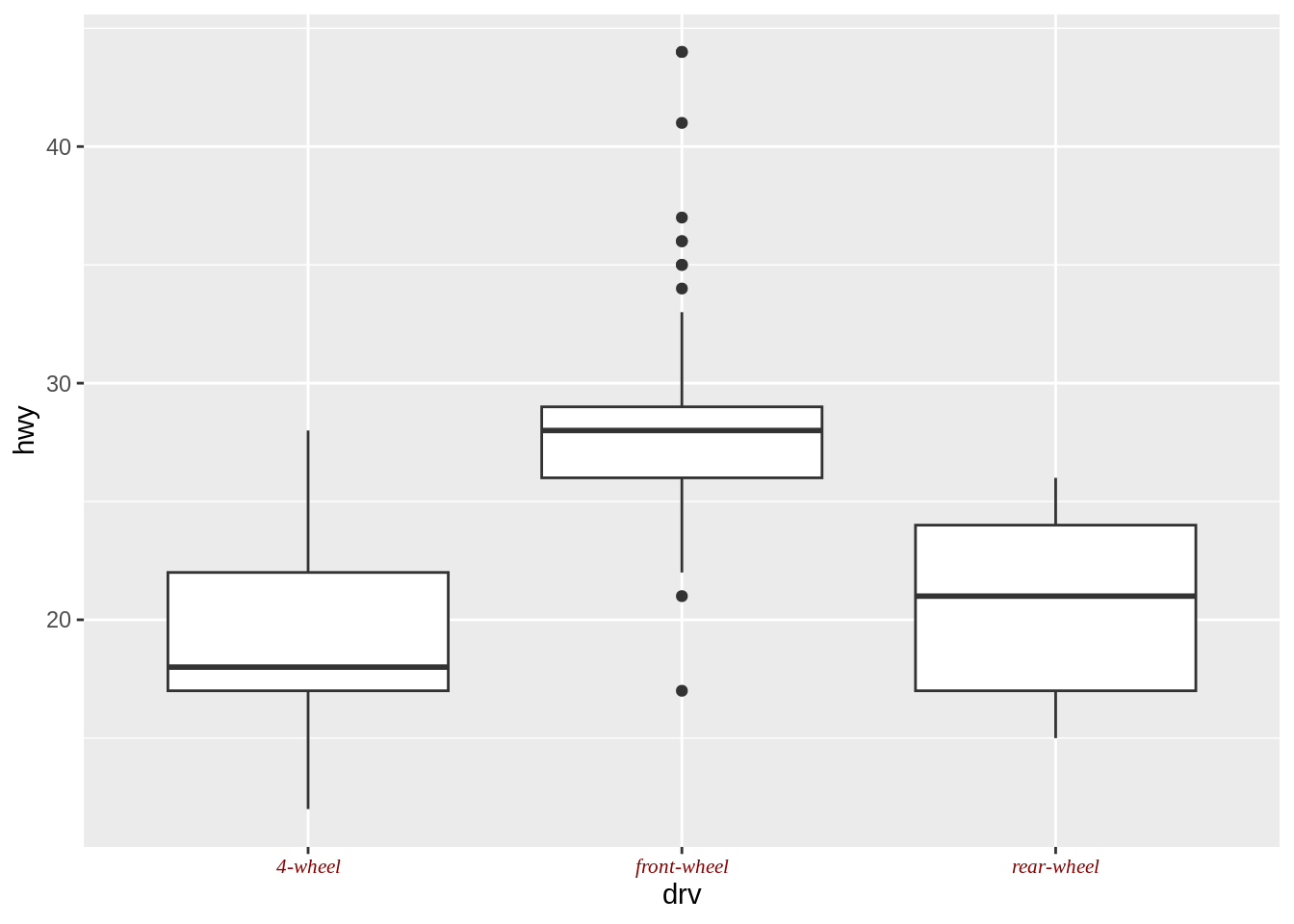

In this example, the size is set to rel(0.9), which means that it is 0.9 times the size of the base font size for the theme.

These commands control the appearance of only the tick labels, on only one axis. They don’t affect the other axis, the axis label, the overall title, or the legend. To control all of these at once, you can use the theming system, which will be discussed later.

Exercise H

Based on the boxplots you created before with the PlantGrowth data,

Change the \(x\)-axis tick labels to “Control”, “Treatment 1”, and “Treatment 2”.

Rotate the text by 45 degrees and make necessary adjustments for both horizontal and vertical alignment, if required.

Switch the font to Helvetica (Mac users) or Times (Non-Mac users), make it bold, and set the font color to “blue”.

35.2.5 Changing the axis labels

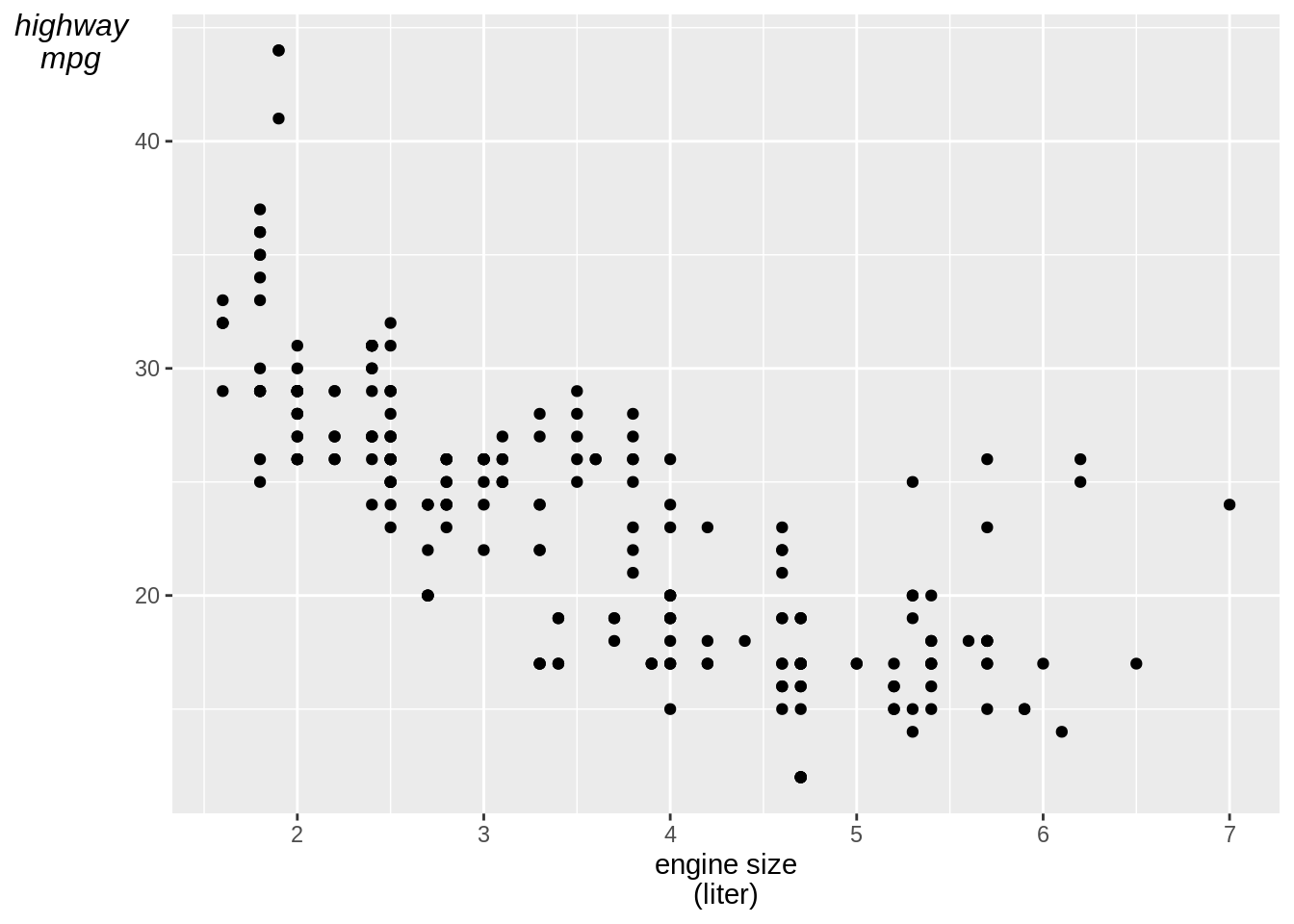
In the previous module, we discussed changing the text of axis labels using xlab() and ylab(). Now let us learn how to modify their appearance.

hwy_plot + 
  xlab("engine size\n(liter)") +
  ylab("highway mpg") +
  theme(axis.title.x = 
          element_text(
            face = "bold", 
            color = "orange", 
            size = 14))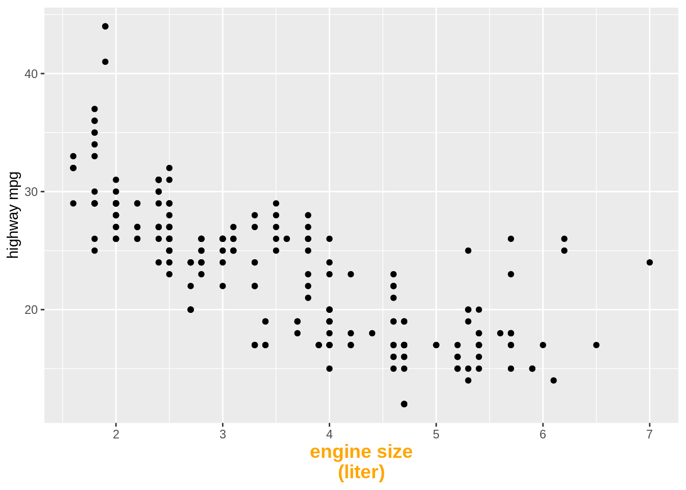

For the \(y\)-axis label, it might also be useful to display the text unrotated:

hwy_plot + 
  xlab("engine size\n(liter)") +
  ylab("highway\nmpg") +
  theme(axis.title.y = 
          element_text(
            angle = 0, 
            face = "italic", 
            size = 12))

35.3 Themes

Here we will discuss how to control the overall appearance of graphics made by ggplot2. The grammar of graphics that underlies ggplot2 is concerned with how data is processed and displayed – it’s not concerned with things like fonts, background colors, and so on. When it comes to presenting your data, there’s a good chance that you’ll want to tune the appearance of these things. ggplot2’s theming system provides control over the appearance of non-data elements. I touched on the theme system in the previous section, and here I’ll explain a bit more about how it works.

35.3.1 Setting the title of a graph

We often want to add a title to our plot. This can be done by ggtitle().

hwy_plot +
  ggtitle("Engine Size and Highway Fuel Economy")

# Use \n for a newline
hwy_plot + 
  ggtitle("Engine Size and \nHighway Fuel Economy")

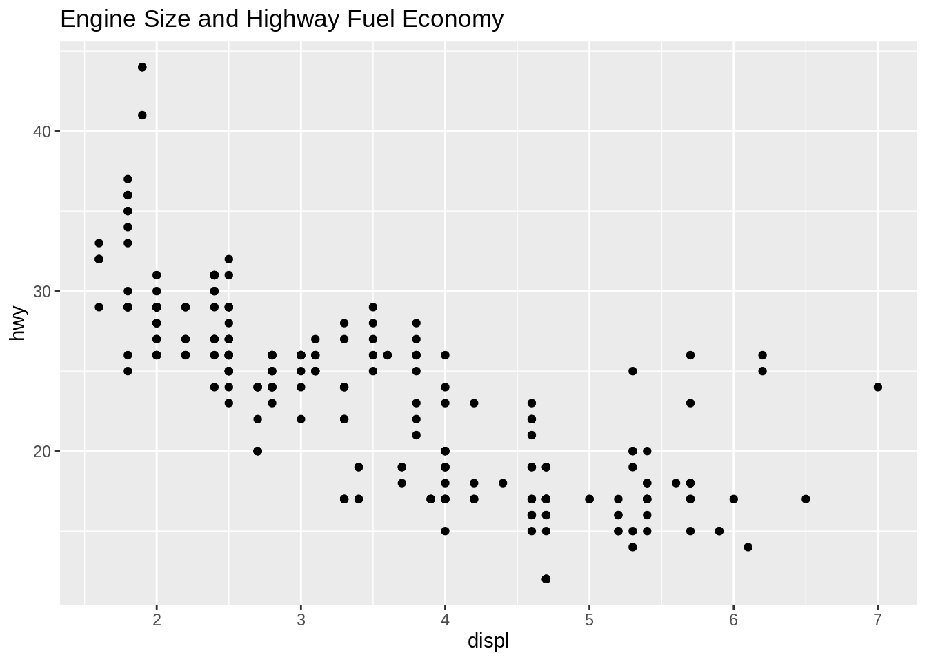
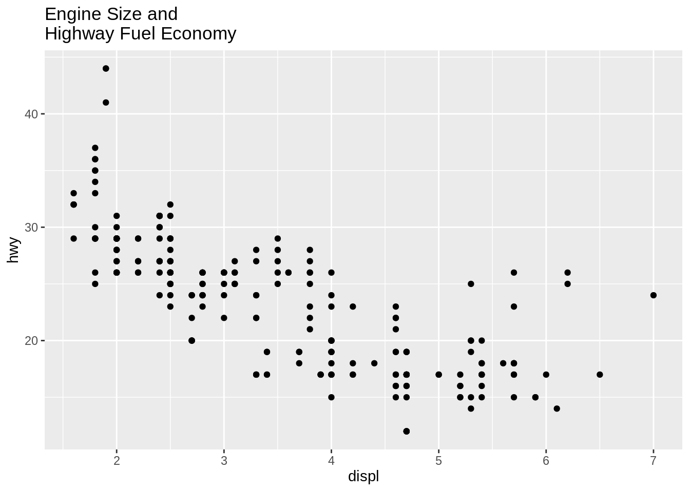
ggtitle() is equivalent to using labs(title = "Title text").

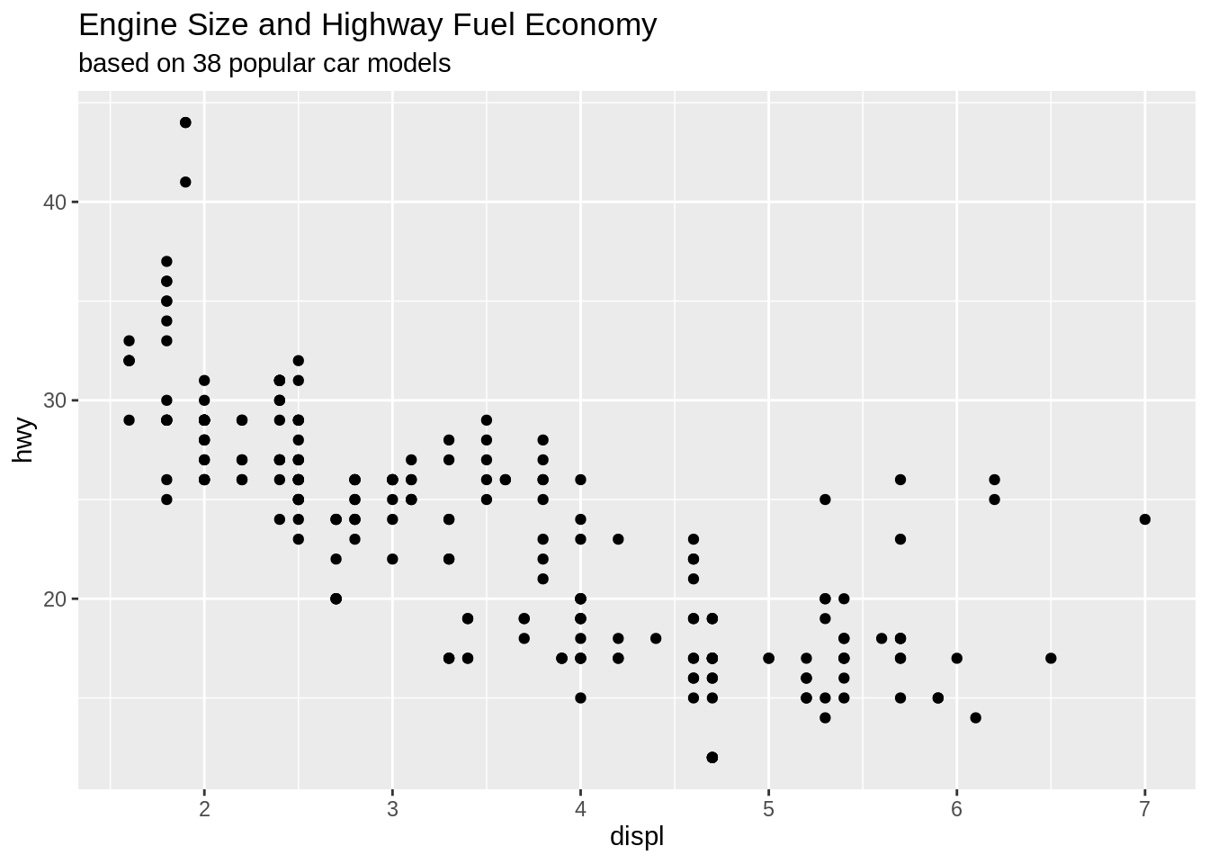
You can add a subtitle by providing a string as the second argument of ggtitle(). By default it will display with slightly smaller text than the main title.

hwy_plot +
  ggtitle("Engine Size and Highway Fuel Economy", "based on 38 popular car models")

35.3.2 Changing the appearance of theme elements

To modify a theme, add theme() with a corresponding element_*() object. These include element_line, element_rect, and element_text.

The following code shows how to modify many of the other commonly used theme properties.

# Options for the plotting area
fueleco_plot +
  theme(
    panel.grid.major = element_line(color = "red"),
    panel.grid.minor = element_line(
      color = "red", linetype = "dashed", linewidth = 0.2),
    panel.background = element_rect(fill = "lightblue"),
    panel.border = element_rect(color = "blue", 
                                fill = NA, linewidth = 2))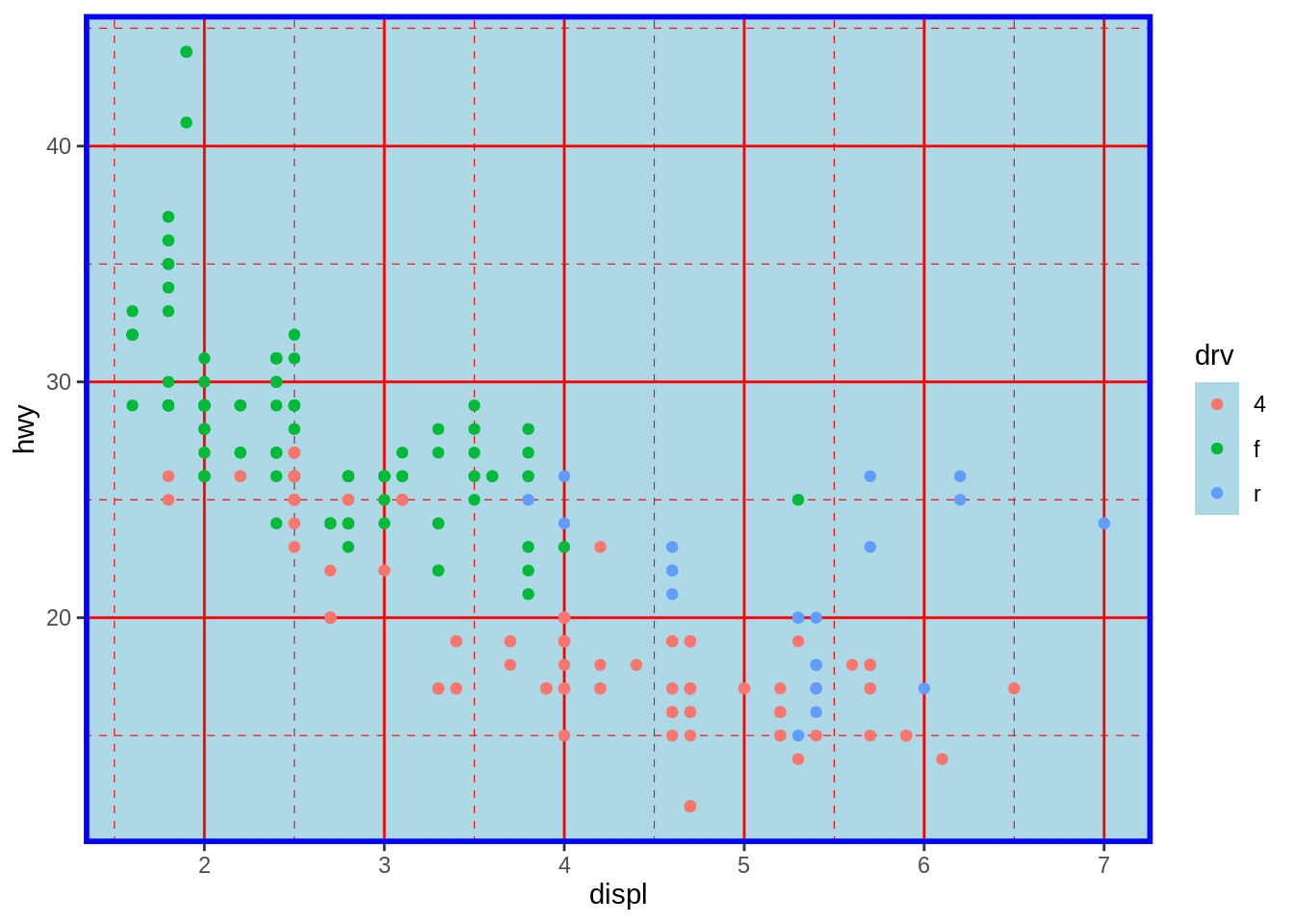

# Options for the legend
fueleco_plot +
  theme(
    legend.background = element_rect(
      fill = "grey85", color = "red", linewidth = 1),
    legend.title = element_text(
      color = "blue", face = "bold", size = 14),
    legend.text = element_text(color = "red"),
    legend.key = element_rect(color = "blue", linewidth = 0.25))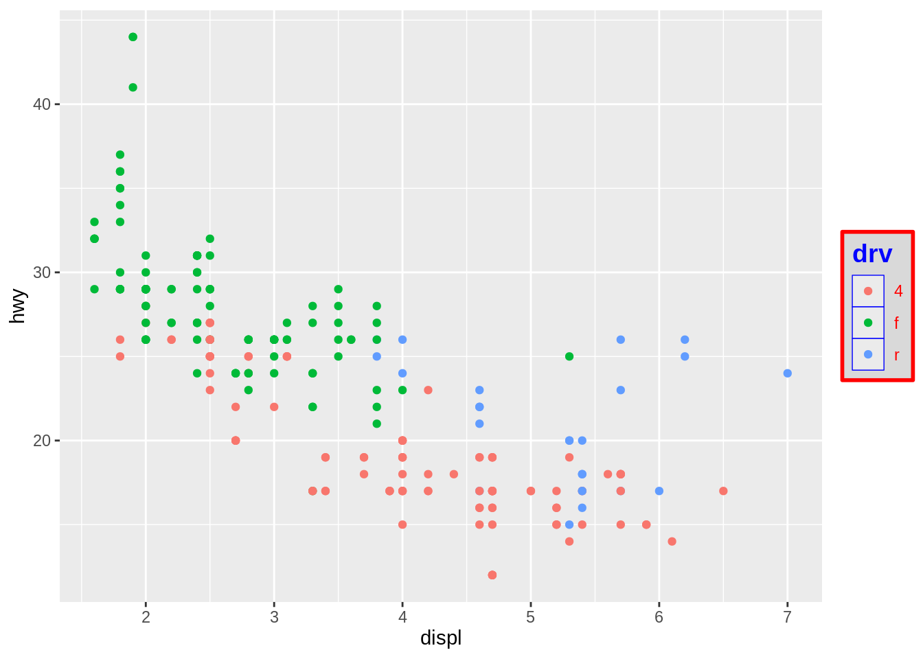

# Options for text items
fueleco_plot +
  ggtitle("Plot title here") +
  theme(
    axis.title.x = element_text(
      color = "red", size = 14),
    axis.text.x  = element_text(color = "blue"),
    axis.title.y = element_text(
      color = "red", size = 14, angle = 90),
    axis.text.y  = element_text(color = "blue"),
    plot.title = element_text(
      color = "red", size = 20, face = "bold"))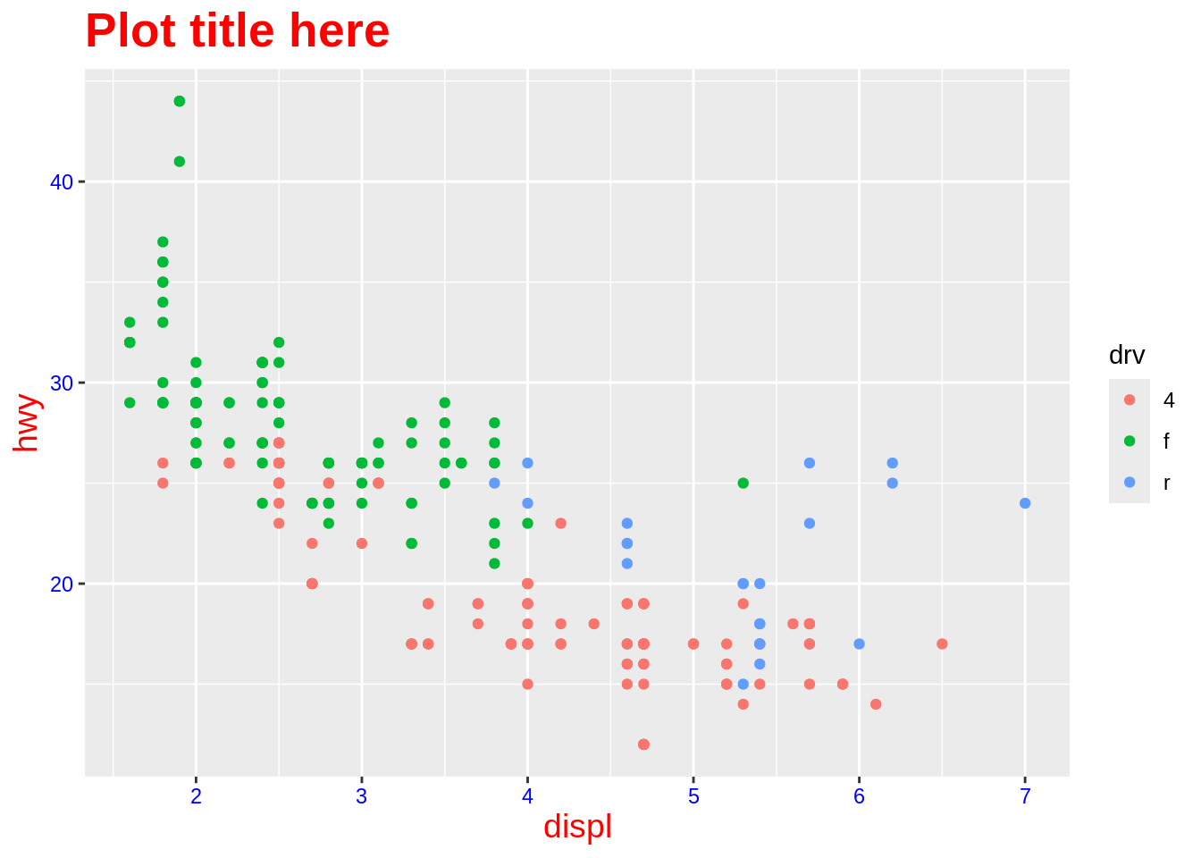

# Options for facets
fueleco_plot +
  facet_grid(drv ~ .) +
  theme(
    strip.background = element_rect(fill = "pink"),
    strip.text.y = element_text(
      size = 14, angle = -90, face = "bold"))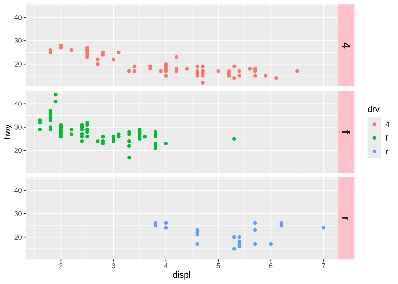

# strip.text.x is the same, but for horizontal facets

More detailed list of theme elements can be found here.

35.3.3 Premade themes

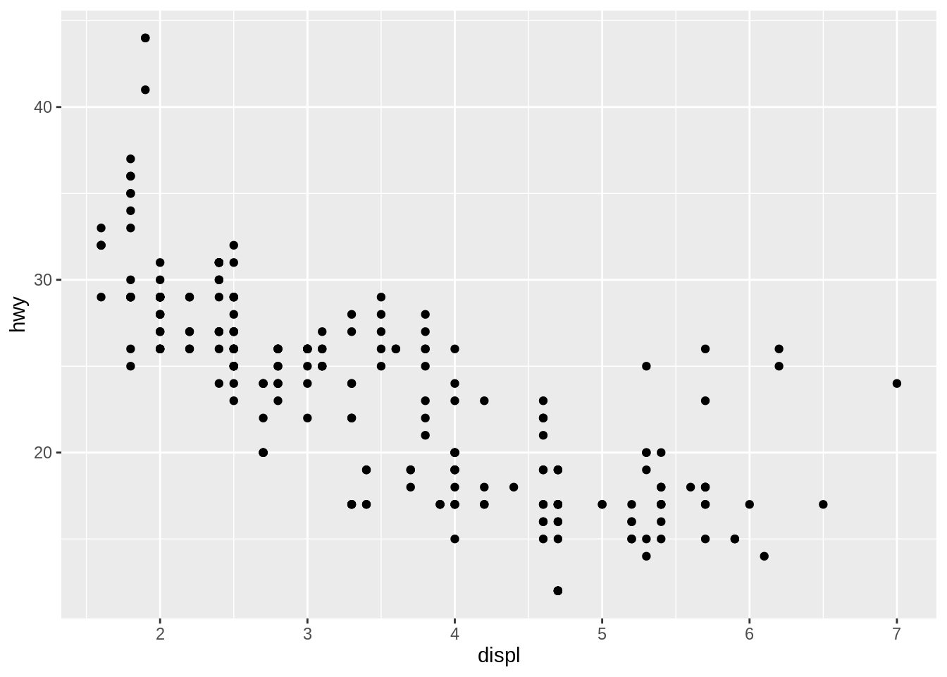
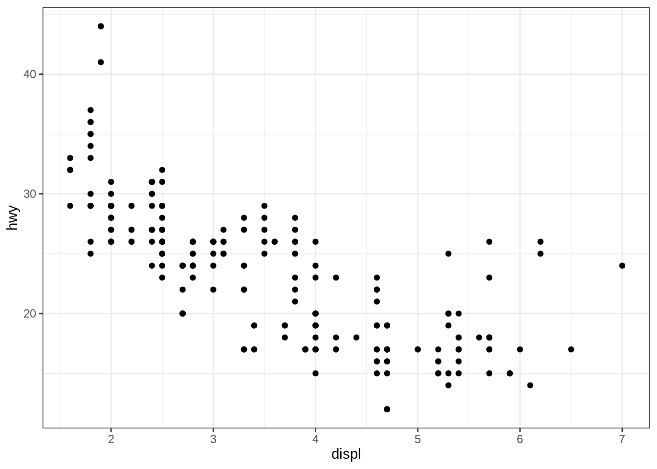
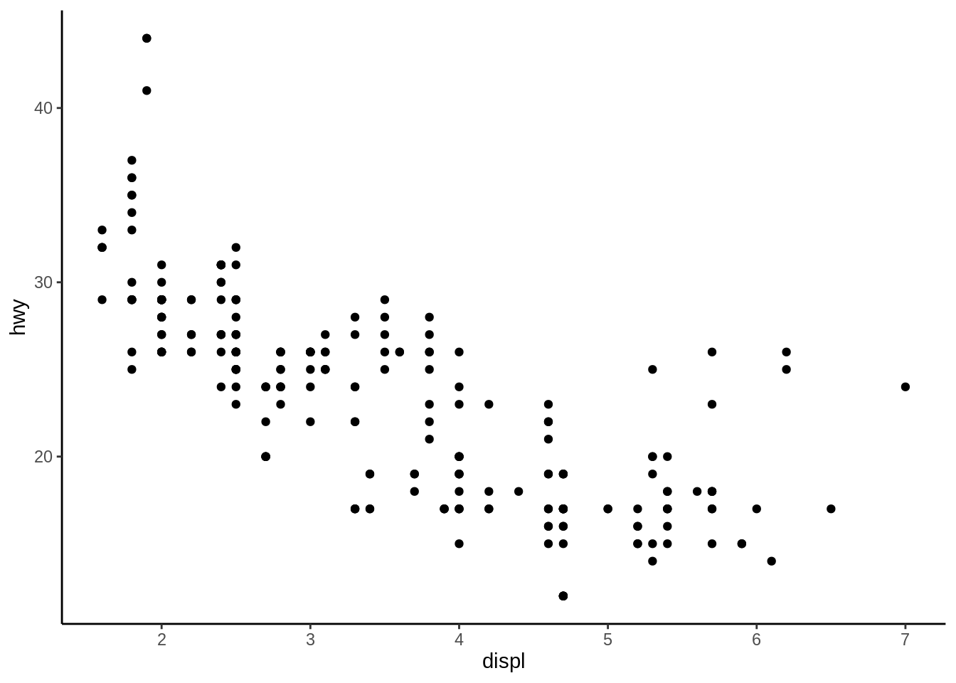
There are many premade themes that are already included in ggplot2. The default ggplot2 theme is theme_grey(), but the examples below also showcase theme_bw(), theme_minimal(), and theme_classic().

# Grey theme (the default)
hwy_plot + theme_grey()

# Black-and-white theme
hwy_plot +
  theme_bw()

# Minimal theme without background annotations
hwy_plot +
  theme_minimal()

# Classic theme, with axis lines but no gridlines
hwy_plot +
  theme_classic()

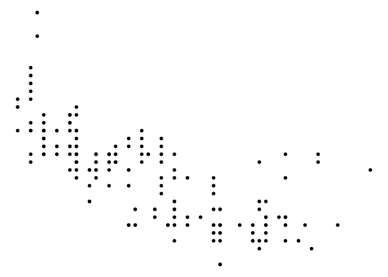
Another theme included in ggplot2 is theme_void(), which makes all plot elements blank and only shows your data. This is especially useful if you don’t want any default theme settings, and instead want a blank slate on which to choose your own theme elements.

hwy_plot +
  theme_void()

Some commonly used properties of theme elements in ggplot2 are those things that are controlled by theme(). Most of these things, like the title, legend, and axes, are outside the plot area, but some of them are inside the plot area, such as grid lines and the background coloring.

Besides the themes included in ggplot2, it is also possible to create your own.

You can set the base font family and size with either of the included themes (the default base font family is Helvetica, and the default size is 12):

hwy_plot +
  theme_grey(base_size = 16, base_family = "Times")

35.4 Legends

Like the \(x\)- or \(y\)-axis, a legend is a guide: it shows people how to map visual (aesthetic) properties back to data values.

35.4.1 Changing the position of a legend

To move the legend from its default place on the right side, we can use theme(legend.position = ...). It can be put on the top, left, right, or bottom by using one of those strings as the position.

fueleco_plot + 
  theme(legend.position = "top")

The legend can also be placed inside the plotting area by specifying a coordinate position, as in legend.position = c(0.9, 0.7). The coordinate space starts at (0, 0) in the bottom left and goes to (1, 1) in the top right.

fueleco_plot + 
  theme(legend.position = c(0.9, 0.7))

Warning: A numeric `legend.position` argument in `theme()` was deprecated in ggplot2
3.5.0.
ℹ Please use the `legend.position.inside` argument of `theme()` instead.

35.4.2 Changing the labels in a legend

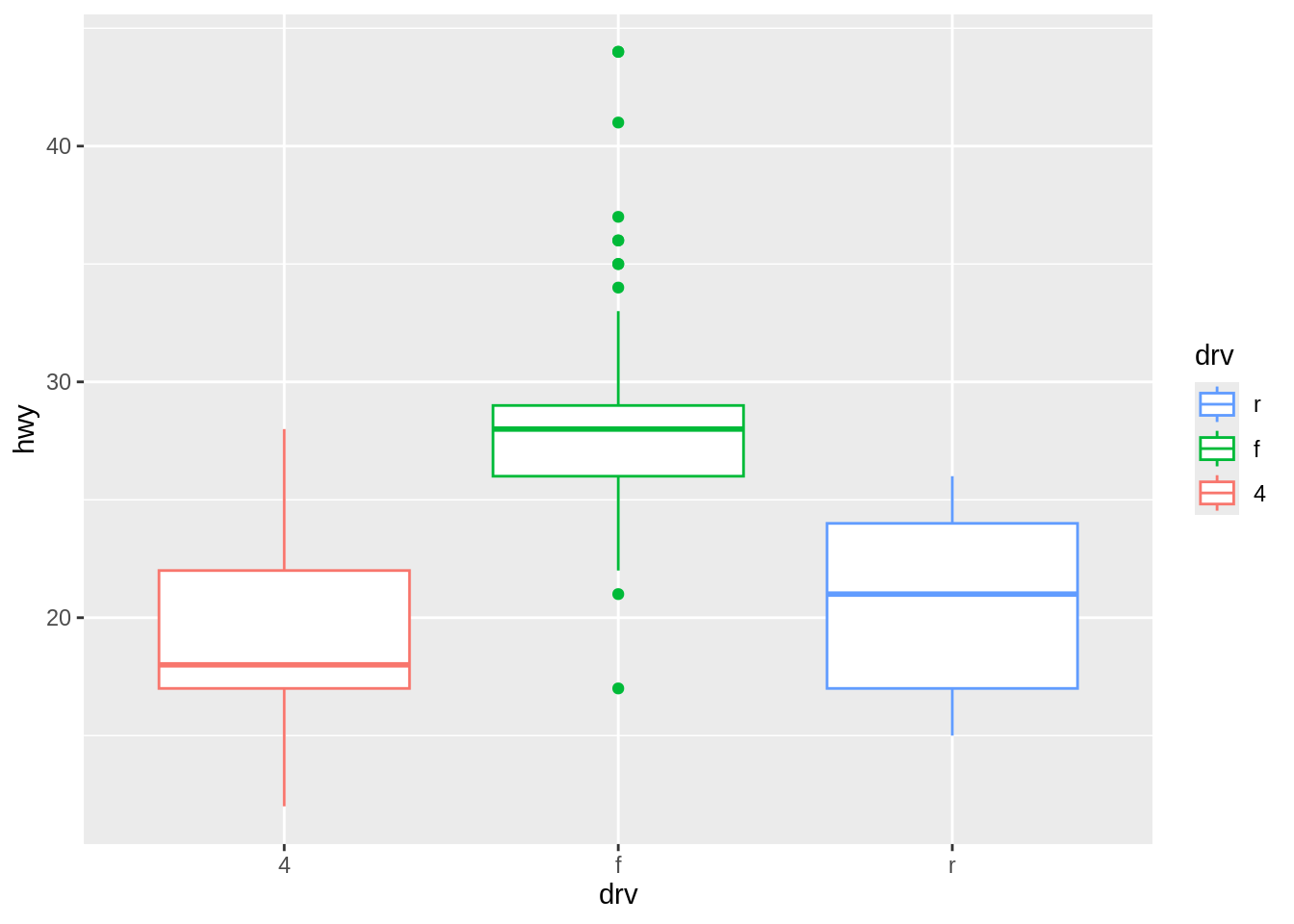
We can change the order of items in a legend by setting the limits in the scale to the desired order.

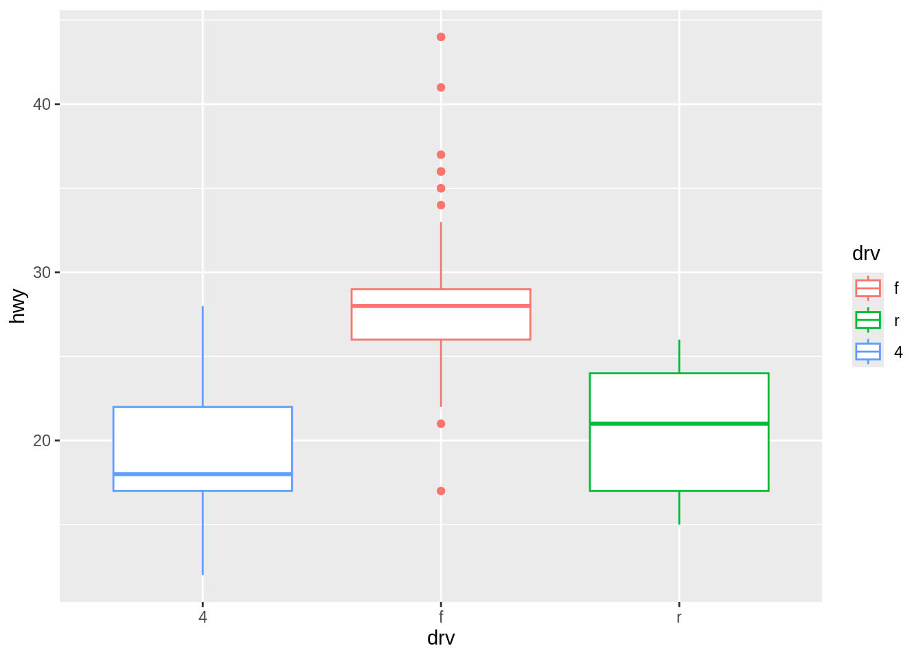
# Create the base plot
mpg_boxplot <- ggplot(mpg, aes(drv, hwy, color = drv)) +
  geom_boxplot()
mpg_boxplot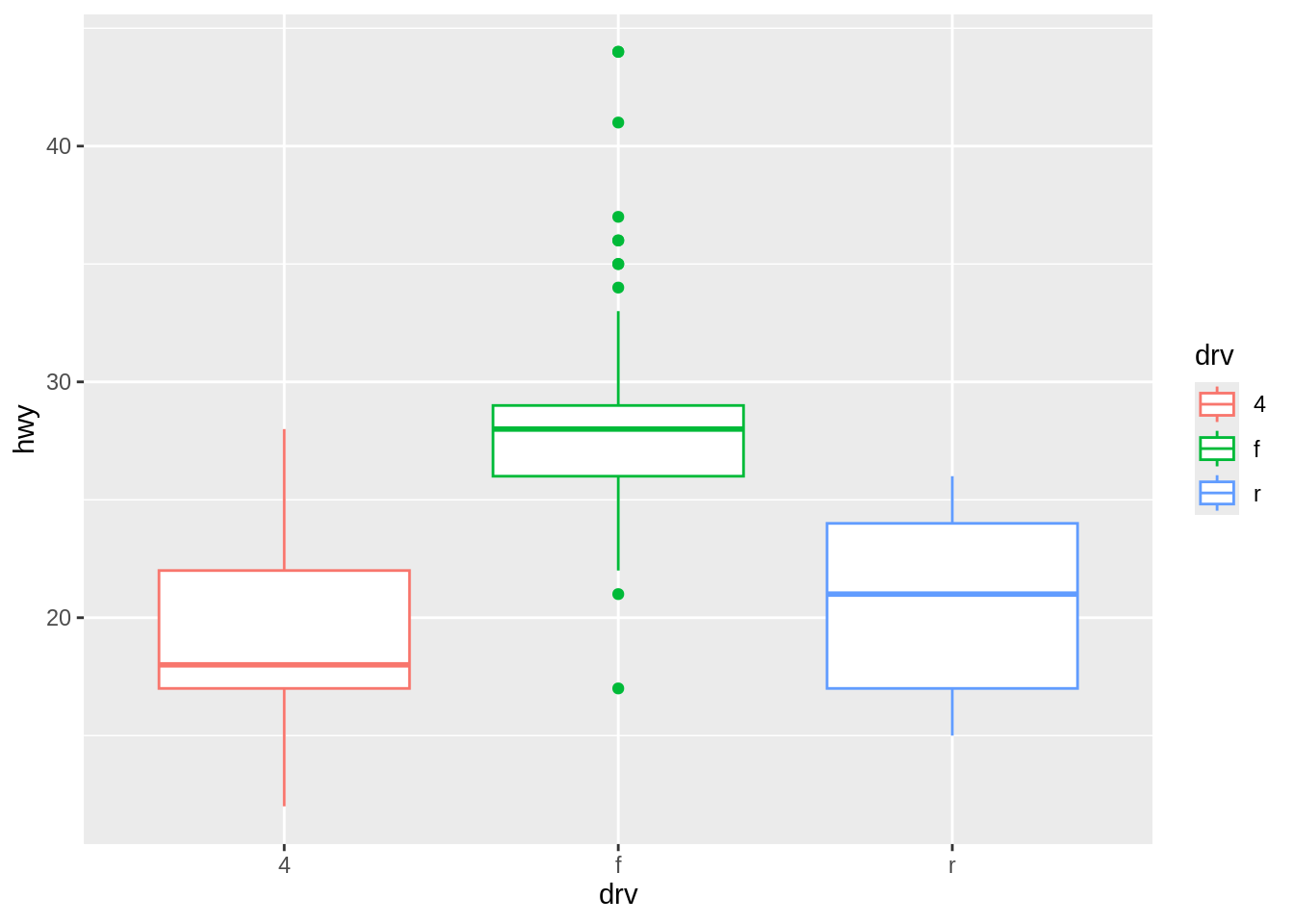

# Change the order of items
mpg_boxplot + 
  scale_color_discrete(limits = c("f", "r", "4"))

Note that the order of the items on the \(x\)-axis did not change. To do that, you would have to set the limits of scale_x_discrete(), or change the data to have a different factor level order.

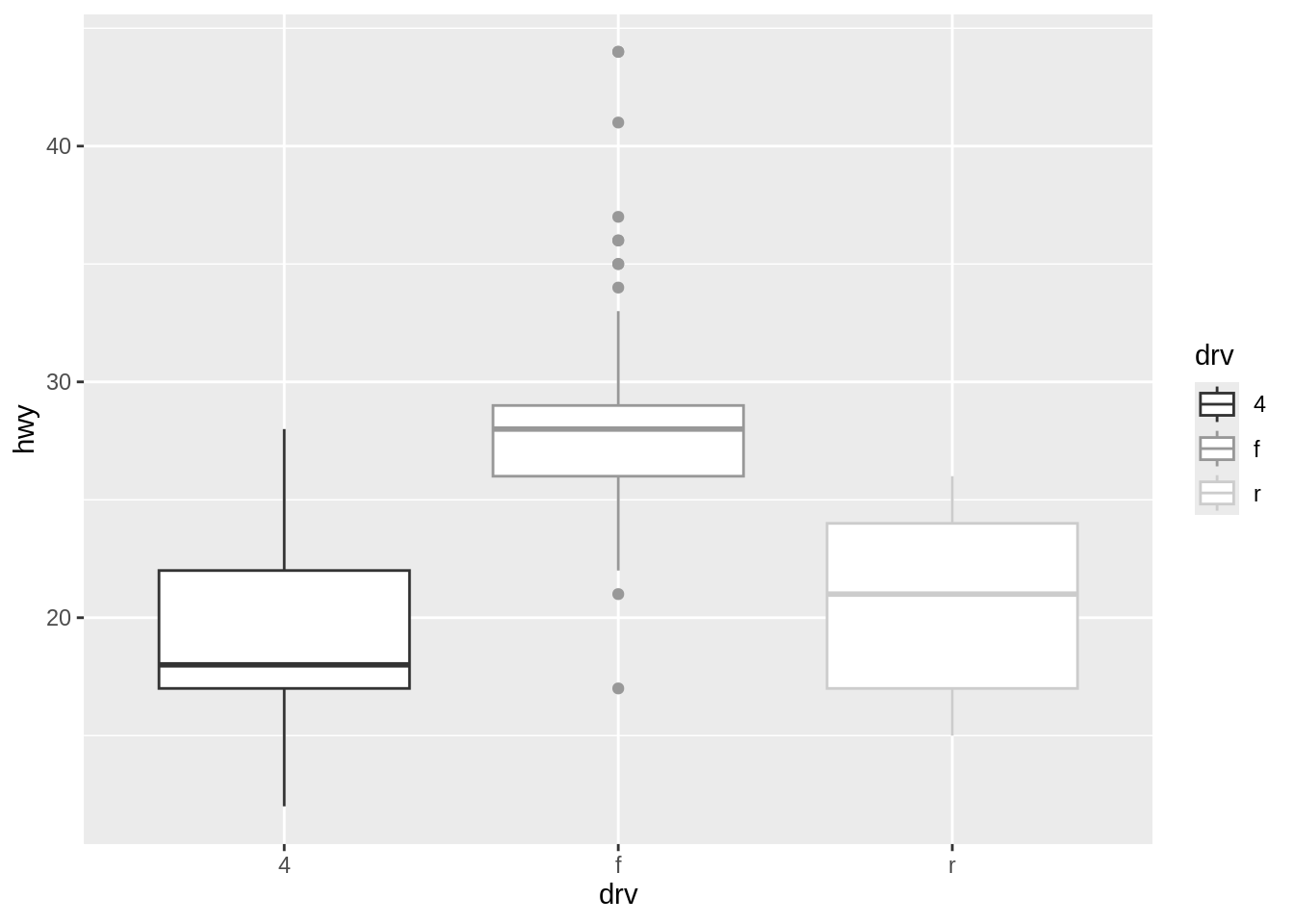
In the preceding example, group was mapped to the color aesthetic. By default this uses scale_color_discrete() (which is the same as scale_color_hue()), which maps the factor levels to colors that are equally spaced around the color wheel. We could have used a different scale_color_*(), though. For example, we could use a grey palette:

mpg_boxplot + 
  scale_color_grey(limits = c("4", "f", "r"))

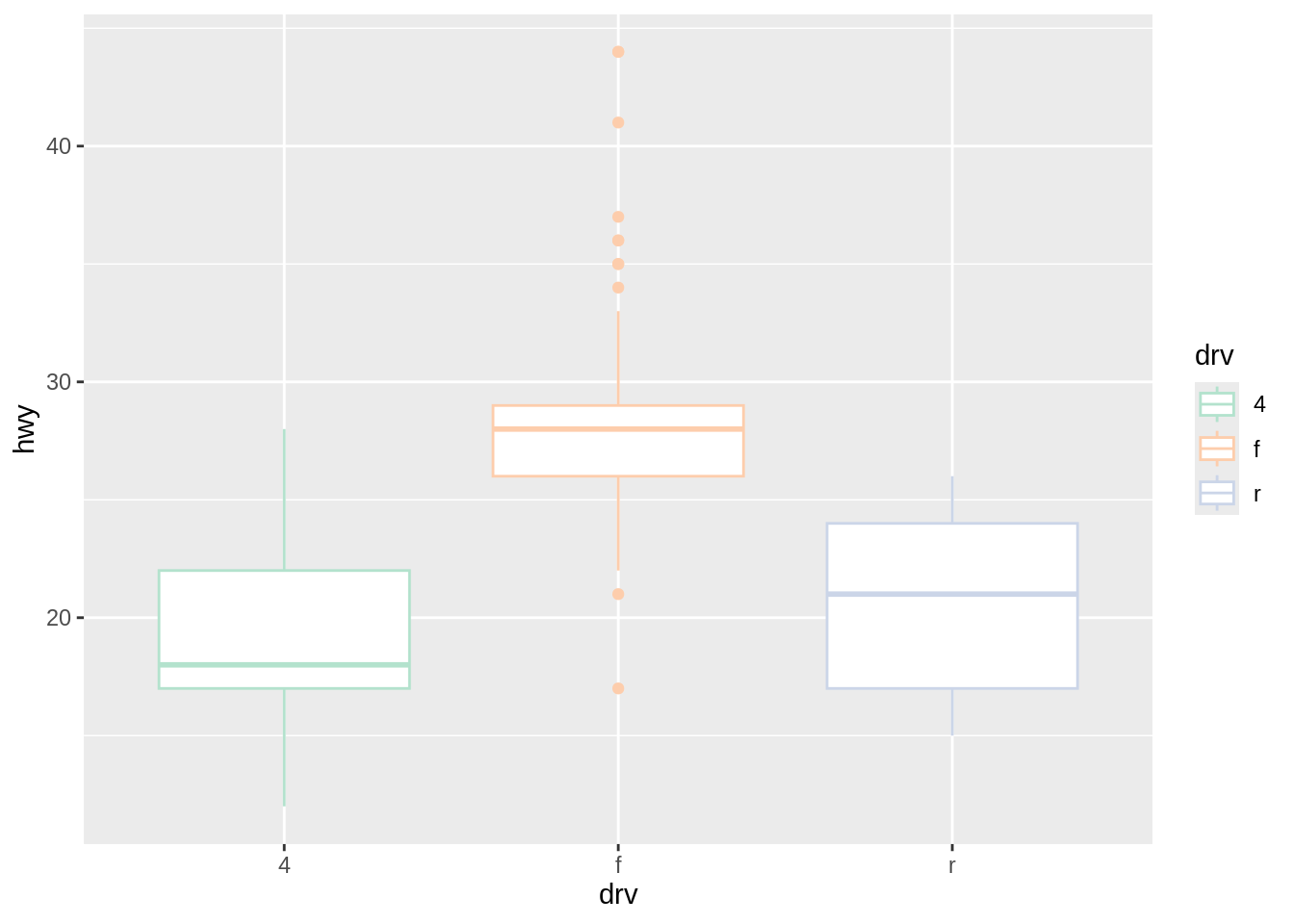
Or we could use a palette from RColorBrewer:

mpg_boxplot + 
  scale_color_brewer(palette = "Pastel2", 
                    limits = c("4", "f", "r"))

All the previous examples were for color. If you use scales for other aesthetics, such as fill (for boxes and bars) or shape (for points), you must use the appropriate scale. Commonly used scales include:

scale_fill_discrete()
scale_fill_hue()
scale_fill_manual()
scale_fill_grey()
scale_fill_brewer()
scale_color_discrete()
scale_color_hue()
scale_color_manual()
scale_color_grey()
scale_color_brewer()
scale_shape_manual()
scale_linetype()

By default, using scale_fill_discrete() is equivalent to using scale_fill_hue(); the same is true for color scales.

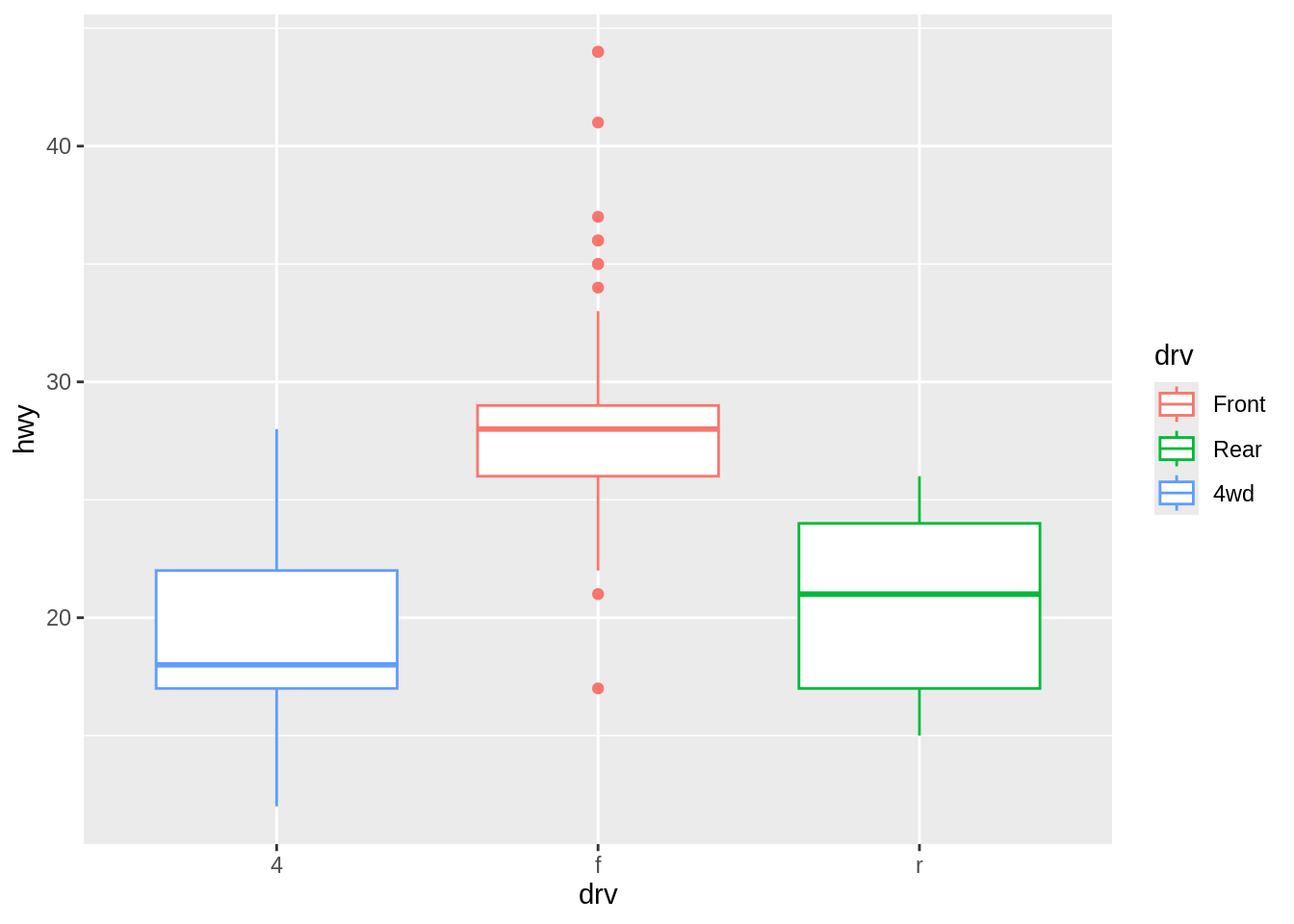
Legend labels can be controlled by these functions as well.

mpg_boxplot + 
  scale_color_discrete(limits = c("f", "r", "4"),
                       labels = c("Front", "Rear", "4wd"))

Exercise I

Attempt to use scale_fill_*() on the previous boxplots. Adjust the labels accordingly, and feel free to rearrange the legend order to your preference.

We can also easily reverse the order of the legend by adding guides (color = guide_legend(reverse = TRUE)).

mpg_boxplot + 
  guides(color = guide_legend(reverse = TRUE))

35.4.3 Changing a legend title

Let us use labs() and set the value of fill, color, shape, or whatever aesthetic is appropriate for the legend. Since legends and axes are both guides, this works the same way as setting the title of the \(x\)- or \(y\)-axis.

ggplot(mpg, aes(displ, hwy, color = drv, size = cyl)) + 
  geom_point() +
  labs(color = "Drive Train", 
       size = "Cylinder")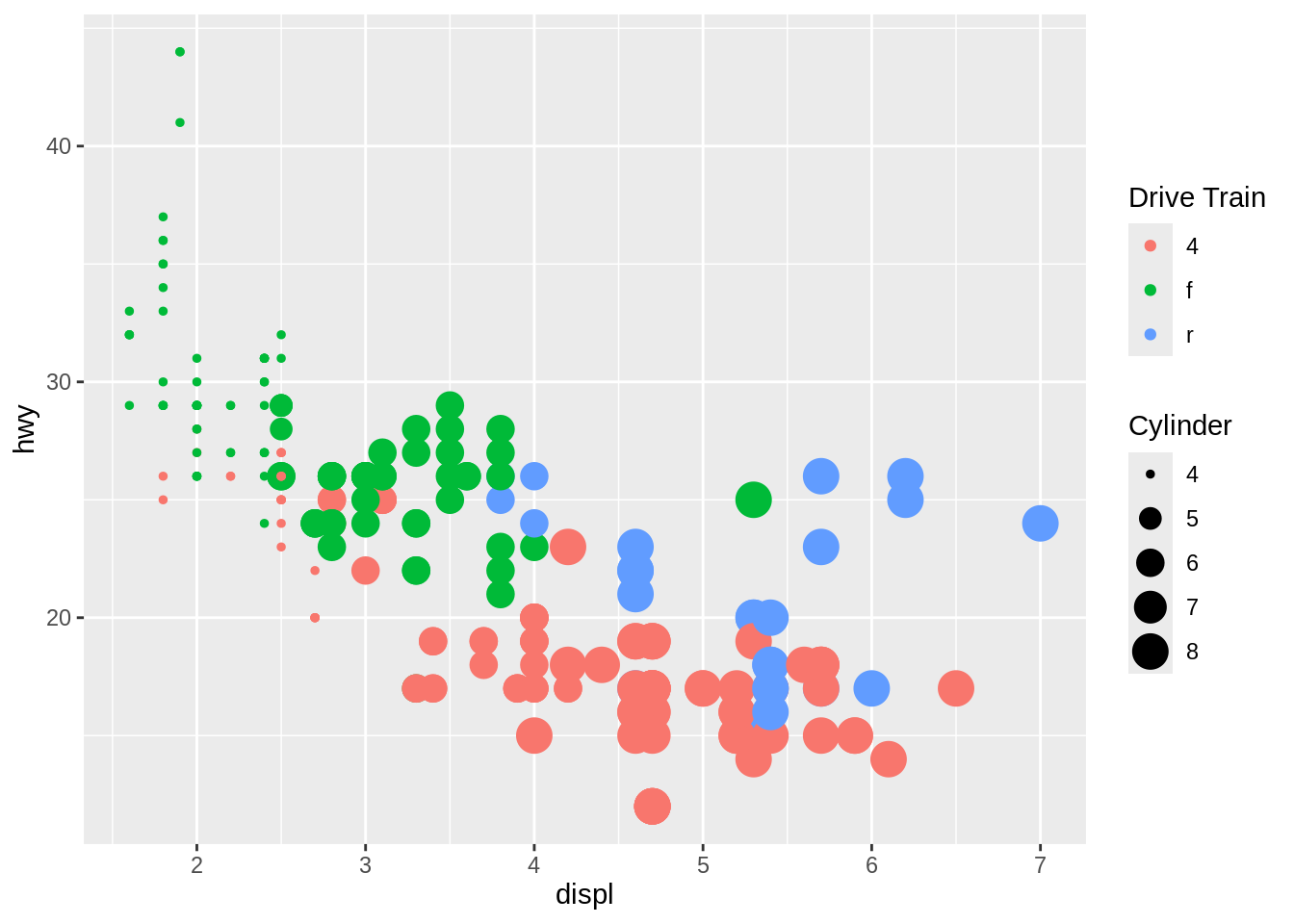

When you want to change the appearance of a legend title’s text, consider using theme(legend.title = element_text().

ggplot(mpg, aes(displ, hwy, color = drv, size = cyl)) +
  geom_point() +
  theme(legend.title = element_text(
    face = "italic",
    family = "Times",
    color = "red",
    size = 14))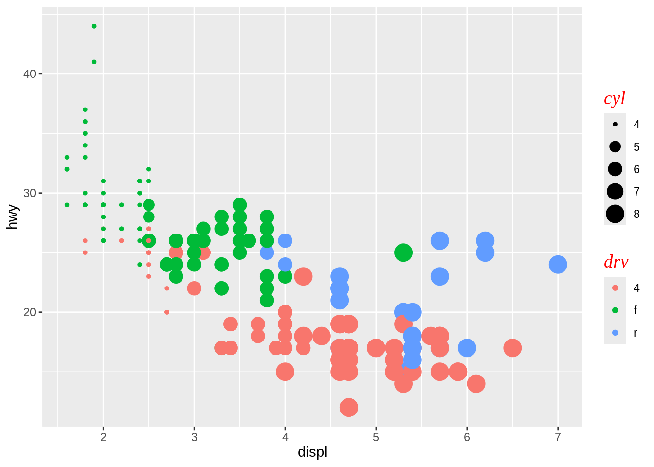

In case you want to remove a legend title, use guides(color = guide_legend(title = NULL)).

ggplot(mpg, aes(displ, hwy, color = drv, size = cyl)) +
  geom_point() + 
  guides(color = guide_legend(title = NULL))