13  Pivot data using tidyr

flowchart TD
  A((tidyr)) -->B{{reshaping}}
  B --> C(pivot_wider):::api
  B --> D(pivot_longer):::api
  classDef api fill:#f96,color:#fff

In addition, we will learn pivoting data using the tidyr package which is also embedded in the meta package tidyverse package.

Let us load the tidyverse package first.

library(tidyverse)

dplyr pairs nicely with tidyr which enables you to swiftly convert between different data formats for plotting and analysis.

The package tidyr addresses the common problem of wanting to reshape your data for plotting and use by different R functions. Sometimes we want data sets where we have one row per observation. Sometimes we want a data frame where each observation type has its own column, and rows are instead more aggregated groups - like surveys, where each column represents an answer. Moving back and forth between these formats is nontrivial, and tidyr gives you tools for this and more sophisticated data manipulation.

To learn more about tidyr, you may want to check out this cheatsheet about tidyr.

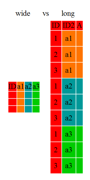
13.1 Long vs Wide table format

The ‘long’ format is where:

• each column is a variable
• each row is an observation

In the ‘long’ format, you usually have 1 column for the observed variable and the other columns are ID variables.

For the ‘wide’ format, a row, for example, could be a research subject for which you have multiple observation variables containing the same type of data, for example responses to a set of survey questions, or repeated observations over time, or a mix of both.

You may find data input to be simpler or some other applications may prefer the ‘wide’ format. However, many of R‘s functions have been designed assuming you have ’long’ format data. This tutorial will help you efficiently transform your data regardless of original format.

The choice of data format affects readability. For humans, the wide format is often more intuitive, since we can often see more of the data on the screen due to its shape. However, the long format is more machine readable and is closer to the formatting of databases. The ID variables in our data frames are similar to the fields in a database and observed variables are like the database values.

13.2 Long to Wide with pivot_wider

Let us see this in action using the built-in data ToothGrowth. We will be using the summary of the data by taking the mean lengths by supplement and doses.

avg_ToothGrowth <- ToothGrowth |> 
  group_by(supp, dose) |> 
  summarise(avg_len = mean(len), .groups = "drop")
avg_ToothGrowth

Now, to make this long data wide, we use pivot_wider from tidyr to turn the supplement types into columns. In addition to our data table we provide pivot_wider with two arguments: names_from describes which column to use for name of the output column, and values_from tells it from column to get the cell values. We’ll use a pipe so we can ignore the data argument.

supp_wide <- avg_ToothGrowth |> 
  pivot_wider(names_from = supp,
              values_from = avg_len)
supp_wide

Exercise F

Q1

Convert avg_ToothGrowth to a wide format by turning dose into columns.

Q2

Work with a built-in data OrchardSprays. Convert this data frame to a wide format by turning treatment into columns.

13.3 Wide to Long with pivot_longer

What if we had the opposite problem, and wanted to go from a wide to long format? For that, we use pivot_longer, which will increase the number of rows and decrease the number of columns. We provide the function with thee arguments: cols which are the columns we want to pivot into the long format, names_to, which is a string specifying the name of the column to create from the data stored in the column names, and values_to, which is also a string, specifying the name of the column to create from the data stored in cell values. So, to go backwards from supp_wide, and exclude dose from the long format, we would do the following:

supp_long <- supp_wide |> 
  pivot_longer(cols = -dose, # exclude the dose column
               names_to = "supp", # name is a string!
               values_to = "avg_len") # also a string
supp_long

We could also have used a specification for what columns to include. This can be useful if you have a large number of identifying columns, and it’s easier to specify what to gather than what to leave alone. And if the columns are adjacent to each other, we don’t even need to list them all out - we can use the : operator!

supp_long <- supp_wide |> 
  pivot_longer(cols = OJ:VC, # columns from OJ to VC
               names_to = "supp",
               values_to = "avg_len")
supp_long

Exercise G

Q1

Convert both data sets you created in Exercise F to a long format.

Q2

Work with the data tidyr::world_bank_pop. Convert it to a long format by turning the years into rows and place them under a column named year. Store population in a new column called population, and name the resulting long data frame pop_long.

13.4 Exporting data

Similar to the read_csv() function used for reading CSV files into R, there is a write_csv() function that generates CSV files from data frames.

Before using write_csv(), make sure you have created an DataOutput folder in the current working directory that will store this generated data set. We don’t want to write generated data sets in the same directory as our raw data. It’s good practice to keep them separate. The Data folder should only contain the raw, unaltered data, and should be left alone to make sure we don’t delete or modify it. In contrast, our script will generate the contents of the DataOutput directory, so even if the files it contains are deleted, we can always re-generate them.

We can now save the table generated above in our DataOutput folder:

write_csv(supp_wide, "DataOutput/supp_wide.csv")