14 Descriptive Statistics
14.1 Exploratory Data Analysis
Every good data analysis begins with a question that you aim to answer using data. As it turns out, there are actually a number of different types of question regarding data: descriptive, exploratory, inferential, predictive, causal, and mechanistic, all of which are defined in the table below.
| Question type | Description | Example |
|---|---|---|
| Descriptive | A question that asks about summarized characteristics of a data set without interpretation (i.e., report a fact). | How many people live in each province and territory in Canada? |
| Exploratory | A question that asks if there are patterns, trends, or relationships within a single data set. Often used to propose hypotheses for future study. | Does political party voting change with indicators of wealth in a set of data collected on 2,000 people living in Canada? |
| Predictive | A question that asks about predicting measurements or labels for individuals (people or things). The focus is on what things predict some outcome, but not what causes the outcome. | What political party will someone vote for in the next Canadian election? |
| Inferential | A question that looks for patterns, trends, or relationships in a single data set and also asks for quantification of how applicable these findings are to the wider population. | Does political party voting change with indicators of wealth for all people living in Canada? |
| Causal | A question that asks about whether changing one factor will lead to a change in another factor, on average, in the wider population. | Does wealth lead to voting for a certain political party in Canadian elections? |
| Mechanistic | A question that asks about the underlying mechanism of the observed patterns, trends, or relationships (i.e., how does it happen?) | How does wealth lead to voting for a certain political party in Canadian elections? |
Prior to diving into data analysis, we usually start off by implementing an Exploratory Data Analysis (EDA) which focuses on addressing descriptive and exploratory questions using descriptive statistics and data visualizations.
14.2 Overview
In this section, we will explore descriptive statistics within the context of a real-world dataset: the Titanic passenger list. We will employ R and various tidyverse functions to manipulate and analyze the data. By the end of this session, you should be able to clean, manipulate, and summarize datasets to reveal insightful trends and patterns.
As part of the EDA, your first step is usually to calculate descriptive statistics from the sample data. These statistics are connected with your underlying research questions and can provide insights to help answer them. In a scientific research report, you might often see a demographic table that serves this purpose.
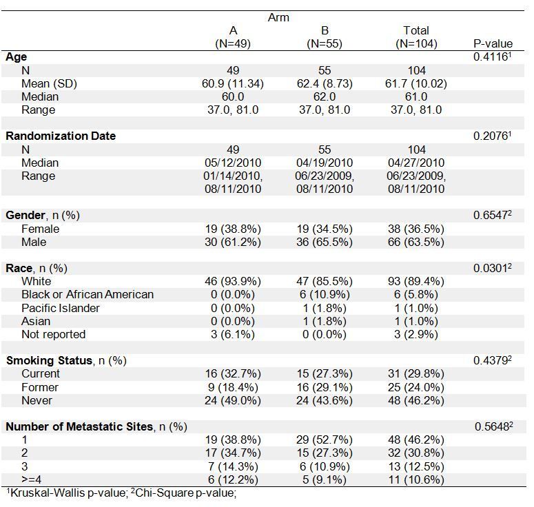
Source: SAS Communities
Once a research question is determined, you will be able to create an informative table. For instance, in the Titanic dataset, one of the research questions is: Are the characteristics of passengers associated with their chances of survival? Therefore, survival status is a key variable under concern, and in what follows, we will concentrate on studying it and its relationship with other variables.
14.3 Understanding Data
The Titanic dataset contains data on the passengers aboard the infamous Titanic ship that sank in 1912. Columns are:
- PassengerId: Identifier of each passenger
- Survived: Survival status (0 = No, 1 = Yes)
- Pclass: Ticket class (1st, 2nd, 3rd)
- Name: Passenger names
- Sex: Gender
- Age: Age in years
- SibSp: Number of Siblings/Spouses Aboard
- Parch: Number of Parents/Children Aboard
- Ticket: Ticket Number
- Fare: Passenger fare
- Cabin: Cabin
- Embarked: Port of Embarkation (C = Cherbourg; Q = Queenstown; S = Southampton)
14.4 Setup
As usual, let us load the packages first.
Load the Titanic training dataset.
14.5 Data Inspection and Cleaning
Before diving into deeper data analysis, it is crucial to first inspect and clean the dataset. This initial step involves checking for inconsistencies, missing values, and outliers that may affect the quality of our insights. By ensuring the data is accurate and well-prepared, we set a solid foundation for more reliable and meaningful exploratory data analysis. In this section, we will walk through the essential processes of data inspection and cleaning, preparing the Titanic dataset for further analysis.
14.5.1 Inspecting Data
Use glimpse() or str() to understand data structure and contents.
Rows: 891
Columns: 12
$ PassengerId <int> 1, 2, 3, 4, 5, 6, 7, 8, 9, 10, 11, 12, 13, 14, 15, 16, 17,…
$ Survived    <int> 0, 1, 1, 1, 0, 0, 0, 0, 1, 1, 1, 1, 0, 0, 0, 1, 0, 1, 0, 1…
$ Pclass      <int> 3, 1, 3, 1, 3, 3, 1, 3, 3, 2, 3, 1, 3, 3, 3, 2, 3, 2, 3, 3…
$ Name        <chr> "Braund, Mr. Owen Harris", "Cumings, Mrs. John Bradley (Fl…
$ Sex         <chr> "male", "female", "female", "female", "male", "male", "mal…
$ Age         <dbl> 22, 38, 26, 35, 35, NA, 54, 2, 27, 14, 4, 58, 20, 39, 14, …
$ SibSp       <int> 1, 1, 0, 1, 0, 0, 0, 3, 0, 1, 1, 0, 0, 1, 0, 0, 4, 0, 1, 0…
$ Parch       <int> 0, 0, 0, 0, 0, 0, 0, 1, 2, 0, 1, 0, 0, 5, 0, 0, 1, 0, 0, 0…
$ Ticket      <chr> "A/5 21171", "PC 17599", "STON/O2. 3101282", "113803", "37…
$ Fare        <dbl> 7.2500, 71.2833, 7.9250, 53.1000, 8.0500, 8.4583, 51.8625,…
$ Cabin       <chr> "", "C85", "", "C123", "", "", "E46", "", "", "", "G6", "C…
$ Embarked    <chr> "S", "C", "S", "S", "S", "Q", "S", "S", "S", "C", "S", "S"…
14.5.2 Cleaning Data
We will focus on handling missing values and formatting variables.
dfm <- dfm |>
  select(-Cabin) |>  # Drop the Cabin column due to high NA
  filter(!is.na(Age)) |>   # Exclude missing Age data
  mutate(PassengerId = as.character(PassengerId), # Convert IDs to strings
         Survived = as.factor(Survived), # Convert Survived to categorical type
         Pclass = as.factor(Pclass), # Convert Pclass to categorical type
         Sex = as.factor(Sex)) # Convert Sex to categorical type
glimpse(dfm)
Rows: 714
Columns: 11
$ PassengerId <chr> "1", "2", "3", "4", "5", "7", "8", "9", "10", "11", "12", …
$ Survived <fct> 0, 1, 1, 1, 0, 0, 0, 1, 1, 1, 1, 0, 0, 0, 1, 0, 0, 0, 1, 1…
$ Pclass <fct> 3, 1, 3, 1, 3, 1, 3, 3, 2, 3, 1, 3, 3, 3, 2, 3, 3, 2, 2, 3…
$ Name <chr> "Braund, Mr. Owen Harris", "Cumings, Mrs. John Bradley (Fl…
$ Sex <fct> male, female, female, female, male, male, male, female, fe…
$ Age <dbl> 22, 38, 26, 35, 35, 54, 2, 27, 14, 4, 58, 20, 39, 14, 55, …
$ SibSp <int> 1, 1, 0, 1, 0, 0, 3, 0, 1, 1, 0, 0, 1, 0, 0, 4, 1, 0, 0, 0…
$ Parch <int> 0, 0, 0, 0, 0, 0, 1, 2, 0, 1, 0, 0, 5, 0, 0, 1, 0, 0, 0, 0…
$ Ticket <chr> "A/5 21171", "PC 17599", "STON/O2. 3101282", "113803", "37…
$ Fare <dbl> 7.2500, 71.2833, 7.9250, 53.1000, 8.0500, 51.8625, 21.0750…
$ Embarked <chr> "S", "C", "S", "S", "S", "S", "S", "S", "C", "S", "S", "S"…To avoid repeated conversions within the mutate() function, we can use the across() function instead.
dfm <- dfm |>
  mutate(PassengerId = as.character(PassengerId), # Convert IDs to strings
         across(c(Survived, Pclass, Sex), as.factor)) # Convert Survived, Pclass and Sex to categorical type
glimpse(dfm)
Rows: 714
Columns: 11
$ PassengerId <chr> "1", "2", "3", "4", "5", "7", "8", "9", "10", "11", "12", …
$ Survived <fct> 0, 1, 1, 1, 0, 0, 0, 1, 1, 1, 1, 0, 0, 0, 1, 0, 0, 0, 1, 1…
$ Pclass <fct> 3, 1, 3, 1, 3, 1, 3, 3, 2, 3, 1, 3, 3, 3, 2, 3, 3, 2, 2, 3…
$ Name <chr> "Braund, Mr. Owen Harris", "Cumings, Mrs. John Bradley (Fl…
$ Sex <fct> male, female, female, female, male, male, male, female, fe…
$ Age <dbl> 22, 38, 26, 35, 35, 54, 2, 27, 14, 4, 58, 20, 39, 14, 55, …
$ SibSp <int> 1, 1, 0, 1, 0, 0, 3, 0, 1, 1, 0, 0, 1, 0, 0, 4, 1, 0, 0, 0…
$ Parch <int> 0, 0, 0, 0, 0, 0, 1, 2, 0, 1, 0, 0, 5, 0, 0, 1, 0, 0, 0, 0…
$ Ticket <chr> "A/5 21171", "PC 17599", "STON/O2. 3101282", "113803", "37…
$ Fare <dbl> 7.2500, 71.2833, 7.9250, 53.1000, 8.0500, 51.8625, 21.0750…
$ Embarked <chr> "S", "C", "S", "S", "S", "S", "S", "S", "C", "S", "S", "S"…Exercise A
Verifying that the data is cleaned: count NA values across all columns.
This code uses the summarize() function along with across() to apply a function across every column in the data frame. everything() function is used to select all columns in the data frame. The function ~sum(is.na(.)) calculates the number of NA values in each column.
14.5.3 Recoding Data
As a last step in cleaning the data, you might find it necessary to recode certain variables to better fit the analytical model or to simplify the analysis.
Recoding involves changing the existing coding of a variable to a new one. For example, in the Titanic dataset, we can recode the Pclass column to consolidate the 2nd and 3rd classes into a single category, distinguishing only between 1st class and non-1st class. Here is how you can do this using the mutate() function along with case_when() from the dplyr package:
# Recode 'Pclass' into two categories and convert to factor
dfm <- dfm |>
  mutate(Pclass_recode = as.factor(case_when(
    Pclass == "1" ~ "First Class", # Classify 1st class as 'First Class'
    Pclass %in% c("2", "3") ~ "Other Classes", # Combine 2nd and 3rd classes as 'Other Classes'
    TRUE ~ NA_character_  # Handles any unexpected cases to NA
  )))
dfm |> select(Pclass, Pclass_recode)
This approach ensures that the original data integrity is preserved (by creating a new column for the recoded data) and that the recoding process is clear and maintainable. Using case_when() allows for complex conditions and multiple recodings in an easily readable format. This is particularly useful when dealing with categorical data that requires consolidation or collapsing for analysis.
Exercise B
14.6 One-Dimensional Descriptive Statistics
If you are interested in summarizing the statistical properties of each column in your dataset, you can use the summary() function. For numeric columns, this function will display a 6-number summary (minimum, 1st quartile, median, mean, 3rd quartile, and maximum). For factor columns, it will show the count of occurrences for each category. Character columns, however, provide limited information - only total counts and the class designation as “character”.
 PassengerId        Survived Pclass      Name               Sex
 Length:714         0:424    1:186   Length:714         female:261
 Class :character   1:290    2:173   Class :character   male  :453
 Mode  :character            3:355   Mode  :character


      Age            SibSp            Parch           Ticket
 Min.   : 0.42   Min.   :0.0000   Min.   :0.0000   Length:714
 1st Qu.:20.12   1st Qu.:0.0000   1st Qu.:0.0000   Class :character
 Median :28.00   Median :0.0000   Median :0.0000   Mode  :character
 Mean   :29.70   Mean   :0.5126   Mean   :0.4314
 3rd Qu.:38.00   3rd Qu.:1.0000   3rd Qu.:1.0000
 Max.   :80.00   Max.   :5.0000   Max.   :6.0000
      Fare          Embarked               Pclass_recode
 Min.   :  0.00   Length:714         First Class  :186
 1st Qu.:  8.05   Class :character   Other Classes:528
 Median : 15.74   Mode  :character
 Mean   : 34.69
 3rd Qu.: 33.38
 Max.   :512.33
Of course, you can calculate additional summary statistics, especially for numeric columns, using the summarize() function. For example:
dfm |> summarize(N = n(),
                 iqr_age = IQR(Age, na.rm = TRUE), # Calculates the Interquartile Range (IQR) for the Age column, ignoring NAs
                 sd_fare = sd(Fare, na.rm = TRUE)) # Calculates the sample standard deviation for the Fare column, ignoring NAs
For categorical variables, we are often more interested in the counts and proportions of the different categories.
dfm |> count(Survived) |> # Count the number of passengers who survived (1) and who did not (0)
  mutate(prop = n / nrow(dfm)) # Divide by the total number of passengers to get proportions
Exercise C
14.7 Two-Dimensional Descriptive Statistics
Usually, it is more insightful to investigate the relationship between two variables during exploratory data analysis. For instance, we can analyze the summary statistics of one variable given the information about another, or examine the distribution of counts based on a subset of data points defined by another variable. These latter variables are often grouping variables, which allow us to obtain grouped summary statistics.
You can start with a grouping variable that is directly connected to your research questions. For example, in the Titanic dataset, our key research question is: Are passenger demographics associated with survival outcomes? Hence, it makes sense to begin with an exploration of the summary data related to Survived.
14.7.1 Numeric Data Summary
We will start by discussing how a numeric variable is associated with Survived.
Summarization: Calculate summary statistics like mean, median, and standard deviation (SD) of Age by survival.
# Calculate summary statistics of Age grouped by survival status
survival_age_summary <- dfm |>
  group_by(Survived) |>
  summarize(avg_age = mean(Age, na.rm = TRUE), # Calculate mean age, ignoring NAs
            med_age = median(Age, na.rm = TRUE), # Calculate median age, ignoring NAs
            sd_age = sd(Age, na.rm = TRUE)) # Calculate standard deviation of age, ignoring NAs
survival_age_summary
For publication purposes, we might prefer to structure these summary statistics in the following way:
# Convert the summary statistics for publication
survival_age_summary_pub <- survival_age_summary |>
  pivot_longer(cols = avg_age:sd_age, # Specify columns to transform from wide to long format
               names_to = "age_stats", # New column to store the names of the original columns
               values_to = "values") |> # New column to store the values from the original columns
  pivot_wider(names_from = Survived, # Use the 'Survived' column to create new columns in the wide format
              values_from = values) # Fill the new columns with corresponding values
survival_age_summary_pub
Exercise D
14.7.2 Categorical Data Summary
Next, we will explore how a categorical variable is associated with Survived.
Grouping Data: Explore the distribution of passengers by sex and survival.
# Count by survival and sex
survival_sex <- dfm |>
group_by(Survived, Sex) |>
summarise(N = n(), .groups = "drop")
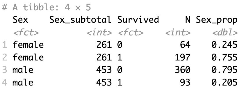
survival_sexWe might be interested in the proportions of females and males in the survived and non-survived groups, respectively.
survival_sex_prop <- survival_sex |>
group_by(Survived) |>
summarize(Sur_subtotal = sum(N)) |> # Obtain subtotals of survived and non-survived passengers, respectively
right_join(survival_sex, by = join_by(Survived)) |> # Merge the subtotals back to the original counts
mutate(Sur_prop = N / Sur_subtotal) # Calculate proportions of females and males within the survived and the non-survived group
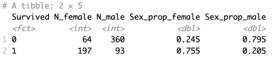
survival_sex_propAgain, for publication purposes, we might want to do the following.
# Prepare survival_sex_prop data for publication by reformatting it
survival_sex_prop_pub <- survival_sex_prop |>
  select(-Sur_subtotal) |> # Remove the Sur_subtotal column as it is no longer needed
  pivot_wider(names_from = "Survived",
              values_from = c(N, Sur_prop)) # Format data to display counts and proportions by survival status
survival_sex_prop_pub
Exercise E
Can you first produce a table similar to the one shown below?
Next, could you convert it to a publishable format as shown below?
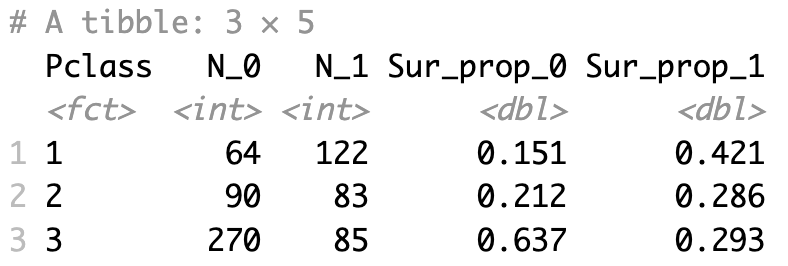
Finally, could you create the table below by investigating the association between Pclass and survival status for publication?
14.8 Three or More - Dimensional Descriptive Statistics
Building on the previous section, we can also extend the summary stats calculation for two or more grouping variables. Making use of the group_by() and summarize() functions, we can, for example, obtain average Age by both Survived and Sex.
Exercise F
Working with three- or higher-dimensional categorical variables involves a more complex structure, but one can start with two-dimensional counts or proportions and extend beyond that.