title: "My report"
execute:
echo: false27 Quarto Basics
27.1 Get Started
Quarto is a command line interface tool, not an R package. This means that help is, by-and-large, not available through ?. Instead, as you work through this chapter, and use Quarto in the future, you should refer to the Quarto Cheatsheet or the Quarto documentation.
You need the Quarto command line interface, but you do not need to explicitly install it or load it, as RStudio automatically does both when needed. The easiest way to create a new quarto document is using the RStudio IDE, i.e., File -> New File -> Quarto Document….
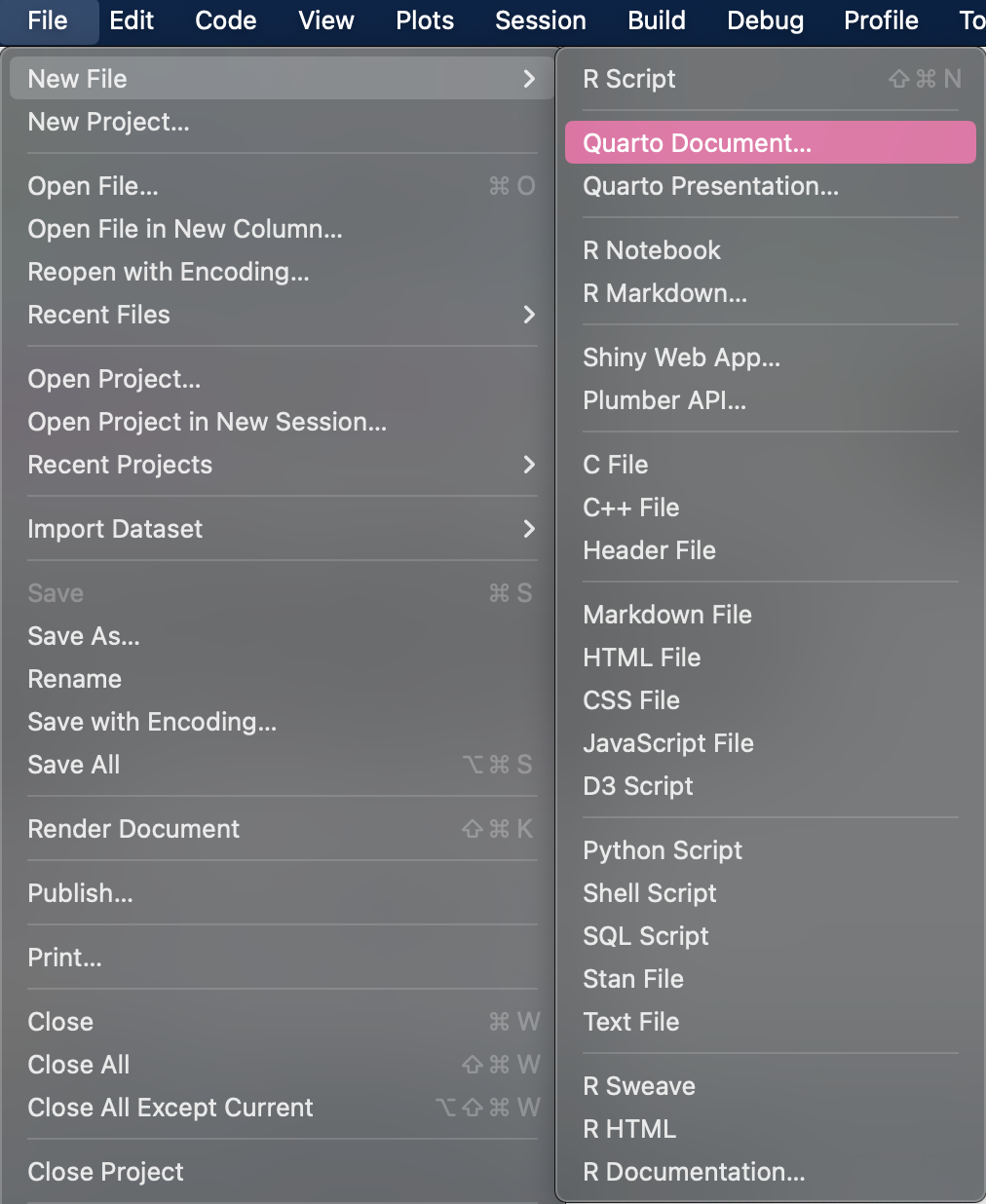
Selecting “Quarto Document…” will lead to the New Quarto Document dialog window, where you can choose the type of desired output document you would like to create. The default option is HTML, which is a good choice if you want to publish your work online or in an email, or if you have not made up your mind yet about how you would like to output your final document. Changing to a different format later is typically as easy as chaining one line of text in the document, or a few clicks in the IDE.
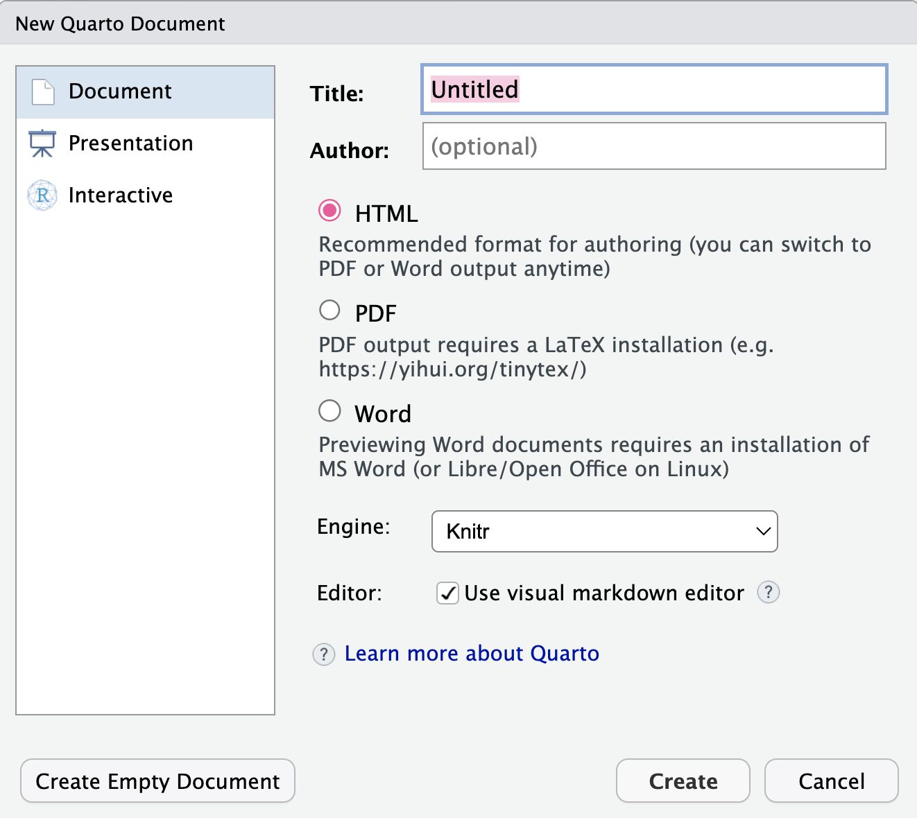
After you make your selection and click Create, you will get a basic quarto template.

A quarto file is a plain text file that has the extension .qmd. See the following example.
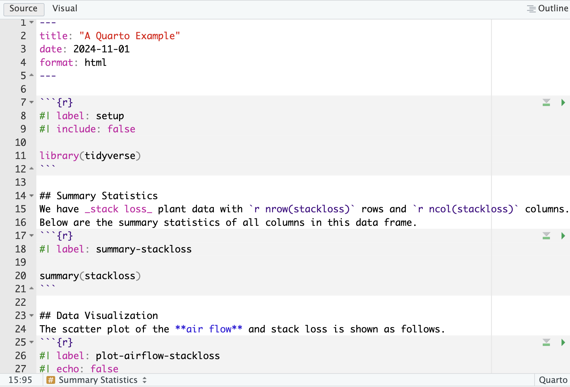
It contains three important types of content:
- An (optional) YAML header surrounded by —s.
- Chunks of R code surrounded by ```.
- Text mixed with simple text formatting like
#heading and_italics_.
It shows a .qmd document in RStudio with notebook interface where code and output are interleaved. You can run each code chunk by clicking the Run icon (it looks like a play button at the top of the chunk), or by pressing Cmd/Ctrl + Shift + Enter. RStudio executes the code and displays the results inline with the code.
To produce a complete report containing all text, code, and results, click Render or press Cmd/Ctrl + Shift + K. You can also do this programmatically with quarto::quarto_render("AQuartoExample.qmd"). This will display the report in the viewer pane and create an HTML file.
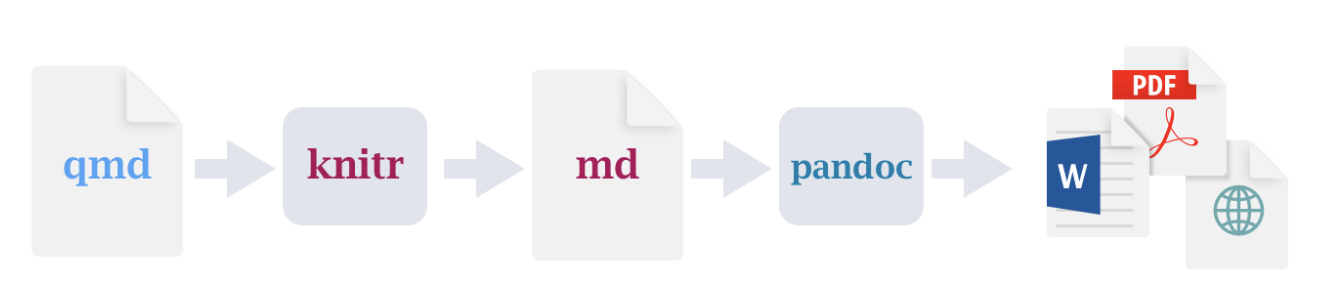
When you render the document, Quarto sends the .qmd file to knitr, https://yihui.org/knitr/, which executes all of the code chunks and creates a new markdown (.md) document which includes the code and its output. The markdown file generated by knitr is then processed by pandoc, https://pandoc.org, which is responsible for creating the finished file. This process is shown in the figure below. The advantage of this two step workflow is that you can create a very wide range of output formats.
Exercise A
27.2 Visual vs. Source Editors
If you are new to computational documents like .qmd files but have experience using tools like Google Docs or MS Word, the easiest way to get started with Quarto in RStudio is the visual editor. The Visual editor in RStudio provides a WYSIWYM interface for authoring Quarto documents. Under the hood, prose in Quarto documents (.qmd files) is written in Markdown, a lightweight set of conventions for formatting plain text files.
In the visual editor you can either use the buttons on the menu bar to insert images, tables, cross-references, etc. or you can use the catch-all Cmd + / or Ctrl + / shortcut to insert just about anything. If you are at the beginning of a line, you can also enter just / to invoke the shortcut. 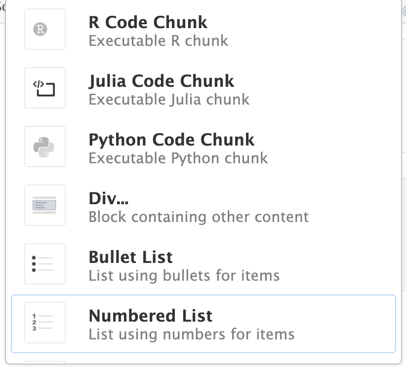
You can also edit Quarto documents using the Source editor in RStudio, without the assist of the Visual editor. While the Visual editor will feel familiar to those with experience writing in tools like Google docs, the Source editor will feel familiar to those with experience writing R scripts or R Markdown documents. The Source editor can also be useful for debugging any Quarto syntax errors since it is often easier to catch these in plain text.
The guide below shows how to use Pandoc’s Markdown for authoring Quarto documents in the source editor.
Text formatting
------------------------------------------------------------

*italic*  or _italic_
**bold**   __bold__
`code`
~~strikeout~~
superscript^2^ and subscript~2~
[underline]{.underline} [small caps]{.smallcaps}

Headings
------------------------------------------------------------

# 1st Level Header

## 2nd Level Header

### 3rd Level Header

Lists
------------------------------------------------------------

-   Bulleted list item 1

-   Item 2

    -   Item 2a

    -   Item 2b

1.  Numbered list item 1

2.  Item 2.
    The numbers are incremented automatically in the output.

Links
------------------------------------------------------------

<http://example.com>

[linked phrase](http://example.com)
The best way to learn these is simply to try them out. It will take a few days, but soon they will become second nature, and you will not need to think about them. If you forget, you can get to a handy reference sheet with Help -> Markdown Quick Reference.
Exercise B
In the previous AQuartoExample.qmd template file we worked with:
27.3 Code Chunks
To run code inside a Quarto document, you need to insert a chunk. There are three ways to do so:
- The keyboard shortcut
Cmd + Option + I(Mac) orCtrl + Alt + I(Windows) - The “+C” icon in the editor toolbar.
- By manually typing the chunk delimiters ```{r} and ```.
It is highly recommended that you learn the keyboard shortcut. It will save you a lot of time in the long run!
You can continue to run the code line by line using the keyboard shortcut that by now: Cmd/Ctrl + Enter. However, chunks get a new keyboard shortcut: Cmd/Ctrl + Shift + Enter, which runs all the code in the chunk. Think of a chunk like a function. A chunk should be relatively self-contained, and focused around a single task.
The following sections describe the chunk header which consists of ```{r}, followed by an optional chunk label and various other chunk options, each on their own line, marked by #|.
27.3.1 Chunk Label
Chunks can be given an optional label, e.g. 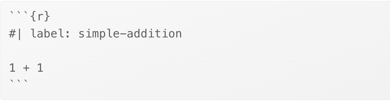
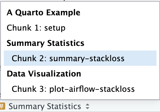
This has three advantages:
- You can more easily navigate to specific chunks using the drop-down code navigator in the bottom-left of the script editor:
Graphics produced by the chunks will have useful names that make them easier to use elsewhere.
You can set up networks of cached chunks to avoid re-performing expensive computations on every run.
Your chunk labels should be short but evocative and should not contain spaces. We recommend using dashes (-) to separate words (instead of underscores, _) and avoiding other special characters in chunk labels.
You are generally free to label your chunk however you like, but there is one chunk name that imbues special behavior: setup. When you are in a notebook mode, the chunk named setup will be run automatically once, before any other code is run.
Additionally, chunk labels cannot be duplicated. Each chunk label must be unique.
Exercise C
27.3.2 Chunk Options
Chunk output can be customized with options, arguments supplied to chunk header. knitr provides almost 60 options that you can use to customize your code chunks. Here we will cover the most important chunk options that you will use frequently. You can see the full list at http://yihui.name/knitr/options/.
The most important set of options controls if your code block is executed and what results are inserted in the finished report:
eval = FALSEprevents code from being evaluated. (And obviously if the code is not run, no results will be generated). This is useful for displaying example code, or for disabling a large block of code without commenting each line.include = FALSEruns the code, but doesn’t show the code or results in the final document. Use this for setup code that you don’t want cluttering your report.echo = FALSEprevents code, but not the results from appearing in the finished file. Use this when writing reports aimed at people who don’t want to see the underlyingRcode.message = FALSEorwarning = FALSEprevents messages or warnings from appearing in the finished file.results = "hide"hides printed output.fig.show = 'hide'hides plots.error = TRUEcauses the render to continue even if code returns an error. This is rarely something you’ll want to include in the final version of your report, but can be very useful if you need to debug exactly what is going on inside your.qmd. It’s also useful if you’re teaching R and want to deliberately include an error. The default,error = FALSEcauses rendering to fail if there is a single error in the document.
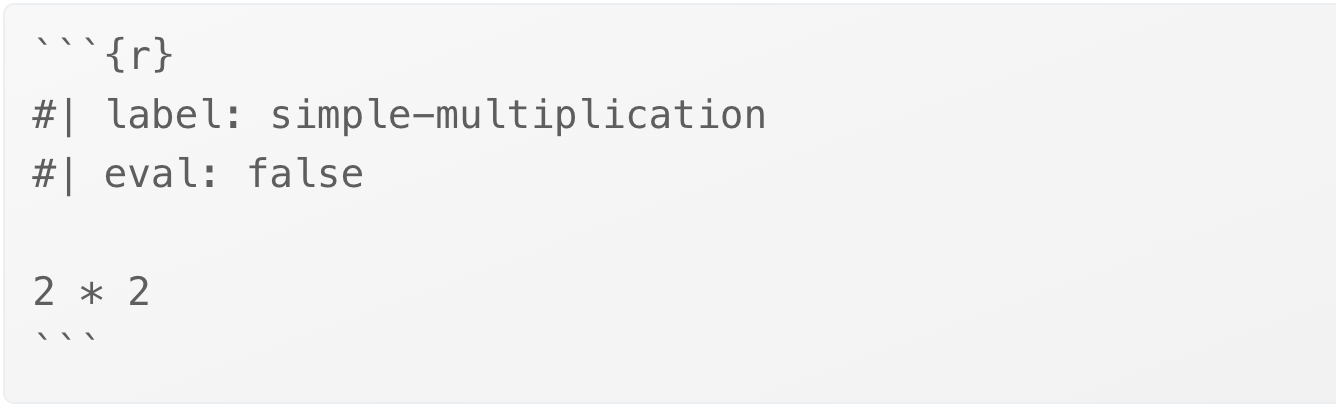
Each of these chunk options get added to the header of the chunk, following #|, e.g., in the following chunk the result is not printed since eval is set to false.
The following table summarizes which types of output each option suppresses:
| Option | Run code | Show code | Output | Plots | Messages | Warnings |
|---|---|---|---|---|---|---|
eval = FALSE |
❌ | ❌ | ❌ | ❌ | ❌ | |
include = FALSE |
❌ | ❌ | ❌ | ❌ | ❌ | |
echo = FALSE |
❌ | |||||
results = "hide" |
❌ | |||||
fig.show = "hide" |
❌ | |||||
message = FALSE |
❌ | |||||
warning = FALSE |
❌ |
Exercise D
27.3.3 Global Options
As you work more with knitr, you will discover that some of the default chunk options do not fit your needs and you want to change them.
You can do this by adding the preferred options in the document YAML, under execute. For example, if you are preparing a report for an audience who does not need to see your code but only your results and narrative, you might set echo: false at the document level. That will hide the code by default, so only showing the chunks you deliberately choose to show (with echo: true). You might consider setting message: false and warning: false, but that would make it harder to debug problems because you would not see any messages in the final document.
Since Quarto is designed to be multi-lingual (works with R as well as other languages like Python, Julia, etc.), all of the knitr options are not available at the document execution level since some of them only work with knitr and not other engines Quarto uses for running code in other languages (e.g., Jupyter). You can, however, still set these as global options for your document under the knitr field, under opts_chunk. For example, when writing books and tutorials we set:
title: "Tutorial"
knitr:
  opts_chunk:
    comment: "#>"
    collapse: true
This uses our preferred comment formatting and ensures that the code and output are kept closely entwined.
Exercise E
27.3.4 Inline code
There is one other way to embed R code into a Quarto document: directly into the text, with: ` r `. This can be very useful if you mention properties of your data in the text. For example, we can write something like:
There are `r
nrow(mtcars)` cars. The mean miles per gallon is `rmean(mtcars$mpg)`.
When the report is rendered, the results of these computations are inserted into the text:
There are 32 cars. The mean miles per gallon is 20.090625.
When inserting numbers into text, format() is your friend. It allows you to set the number of digits so you don’t print to a ridiculous degree of precision, and a big.mark to make numbers easier to read.
Hence, we can write:
There are 32 cars. The mean miles per gallon is 20.1.