18 Geometrics

Tip

flowchart LR
  AC{{Geometries}}
  AC -->ACA(geom_point)
  AC -->ACB(geom_line)
  AC -->ACC(geom_bar)
  AC -->ACD(geom_histogram)
  AC -->ACE(geom_boxplot)
  AC -->ACF(geom_smooth)
  AC -->ACG(geom_freqpoly)
  AC -->ACH(geom_density)

library(tidyverse)

In the previous module, we have learned geom_point(), geom_line(), geom_bar(), geom_histogram(), geom_boxplot(). Here let us explore more geom_*() functions.

18.1 Adding a smoother to a plot

If you have a scatterplot with a lot of noise, it can be hard to see the dominant pattern. In this case it’s useful to add a smoothed line to the plot with geom_smooth(), which fits a smoother to the data and displays the smooth and its standard error.

ggplot(mpg, aes(x = displ, y = hwy)) + 
  geom_point() + 
  geom_smooth()

`geom_smooth()` using method = 'loess' and formula = 'y ~ x'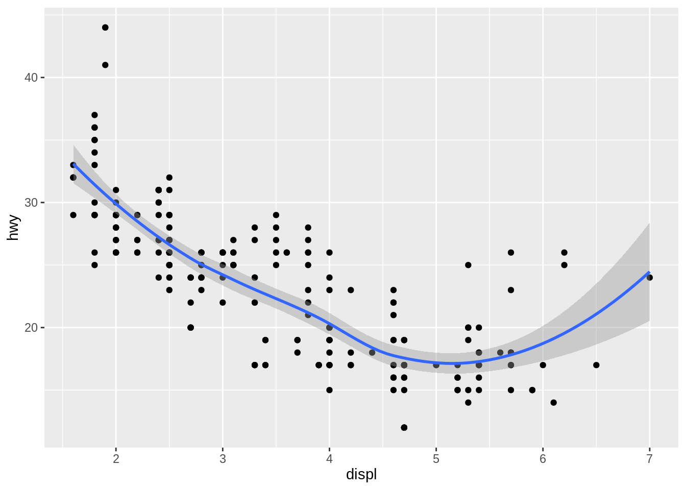

This overlays the scatterplot with a smooth curve, including an assessment of uncertainty in the form of point-wise confidence intervals shown in grey. If you’re not interested in the confidence interval, turn it off with geom_smooth(se = FALSE).

An important argument to geom_smooth() is the method, which allows you to choose which type of model is used to fit the smooth curve:

method = "loess", the default for small \(n\), uses a smooth local regression (as described in ?loess). The wiggliness of the line is controlled by the span parameter, which ranges from 0 (exceedingly wiggly) to 1 (not so wiggly).

ggplot(mpg, aes(x = displ, y = hwy)) + 
  geom_point() + 
  geom_smooth(method = "loess", formula = y ~ x, span = 0.2)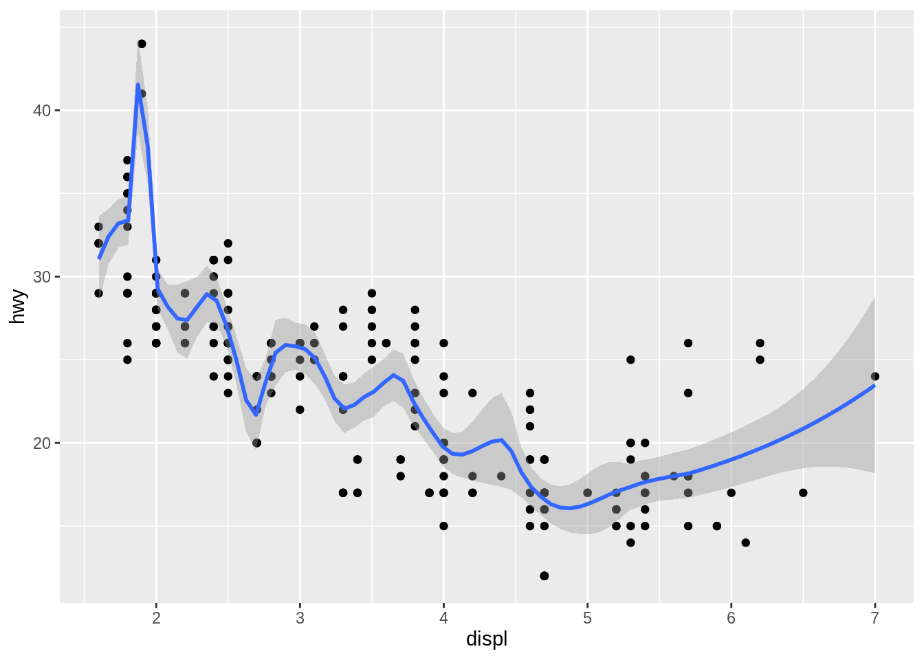

ggplot(mpg, aes(x = displ, y = hwy)) + 
  geom_point() + 
  geom_smooth(method = "loess", formula = y ~ x, span = 1)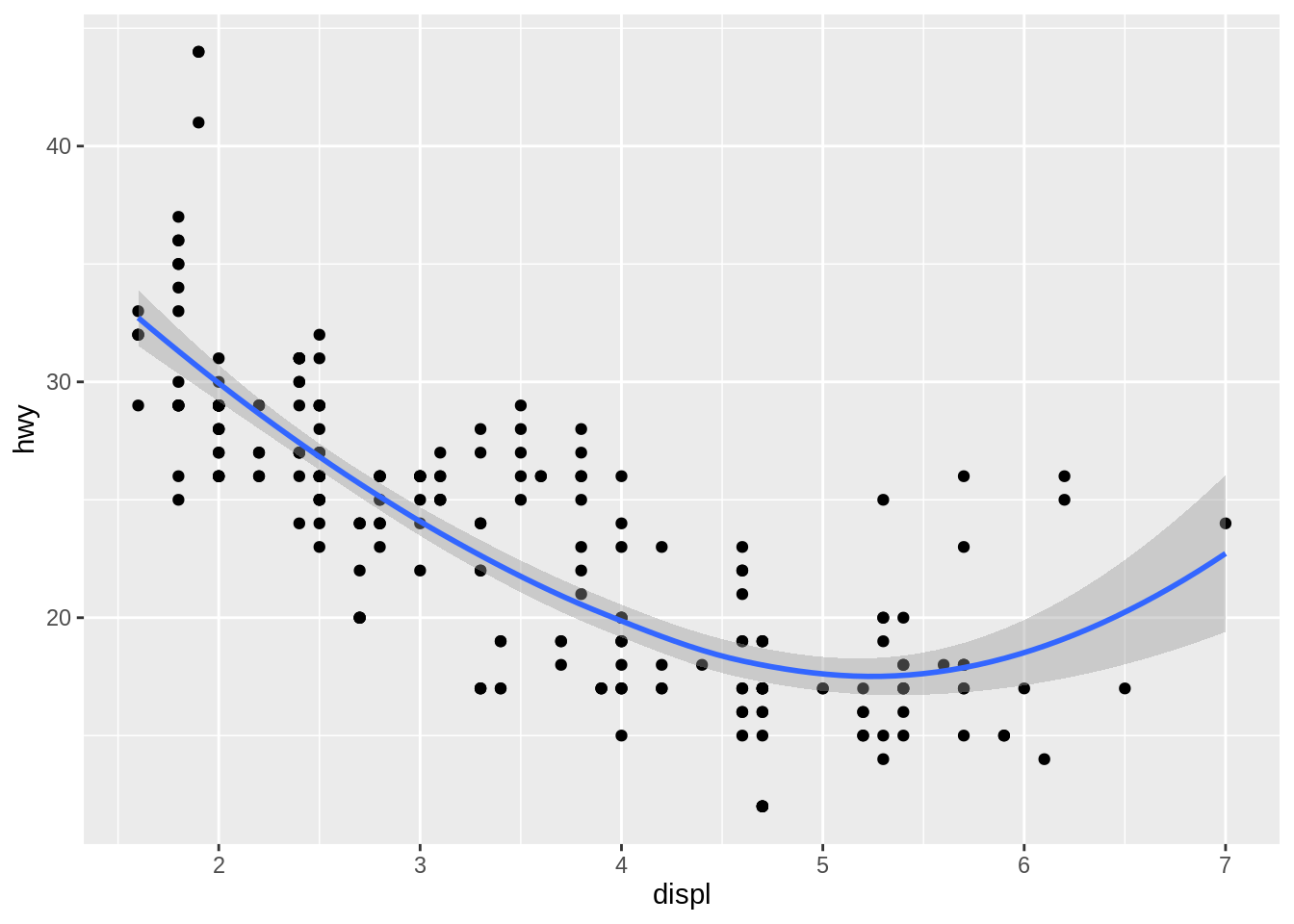

loess does not work well for large data sets, so an alternative smoothing algorithm is used when \(n\) is greater than 1,000.

method = "gam" fits a generalized additive model provided by the mgcv package. You need to first load mgcv, then use a formula like formula = y ~ s(x) or y ~ s(x, bs = "cs") (for large data). This is what ggplot2 uses when there are more than 1,000 points.

library(mgcv)
ggplot(mpg, aes(x = displ, y = hwy)) + 
  geom_point() + 
  geom_smooth(method = "gam", formula = y ~ s(x))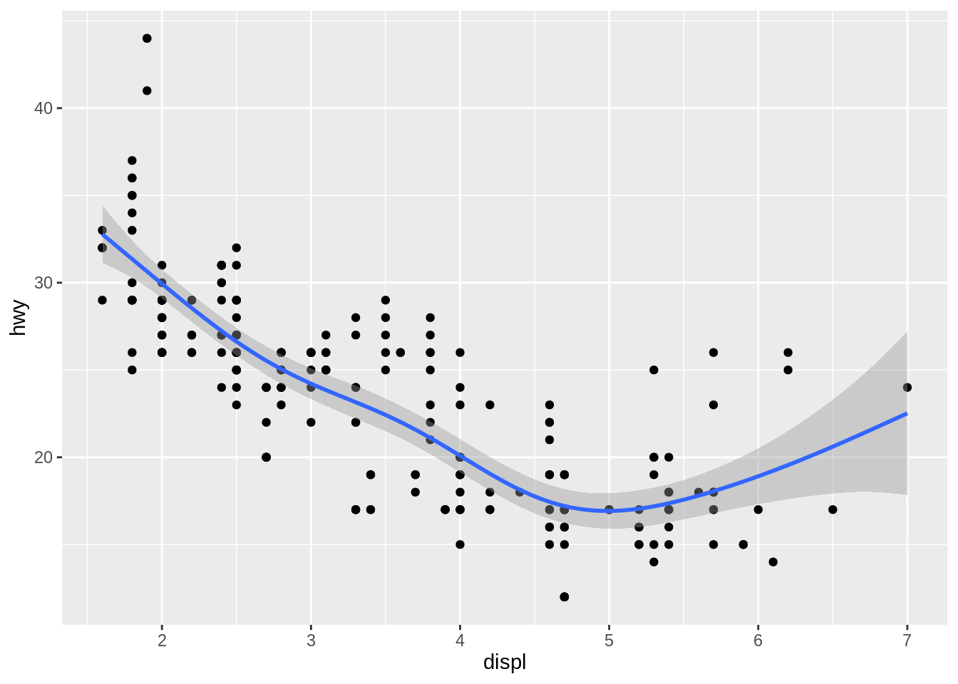

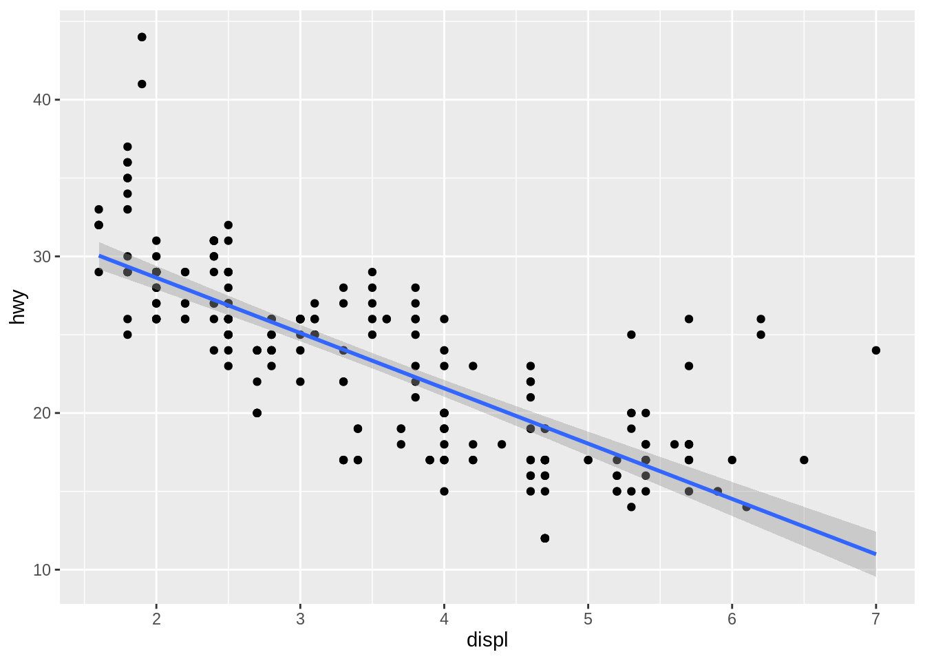
method = "lm" fits a linear model, giving the line of best fit.

ggplot(mpg, aes(x = displ, y = hwy)) + 
  geom_point() + 
  geom_smooth(method = "lm", formula = y ~ x)

method = "rlm" works like lm(), but uses a robust fitting algorithm so that outliers don’t affect the fit as much. It’s part of the MASS package, so remember to load that first.

library(MASS)
ggplot(mpg, aes(x = displ, y = hwy)) + 
  geom_point() + 
  geom_smooth(method = "rlm", formula = y ~ x)

Exercise D

Add a smoother to the scatterplot addressing the relationship between cty and displ. You may explore different methods.

18.2 Histograms and frequency polygons

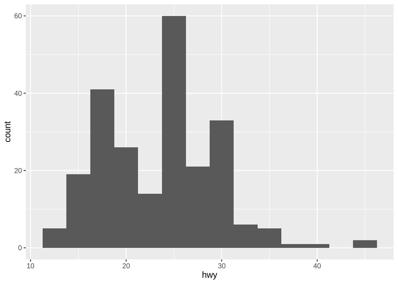
Histograms and frequency polygons show the distribution of a single numeric variable. They provide more information about the distribution of a single group than boxplots do, at the expense of needing more space.

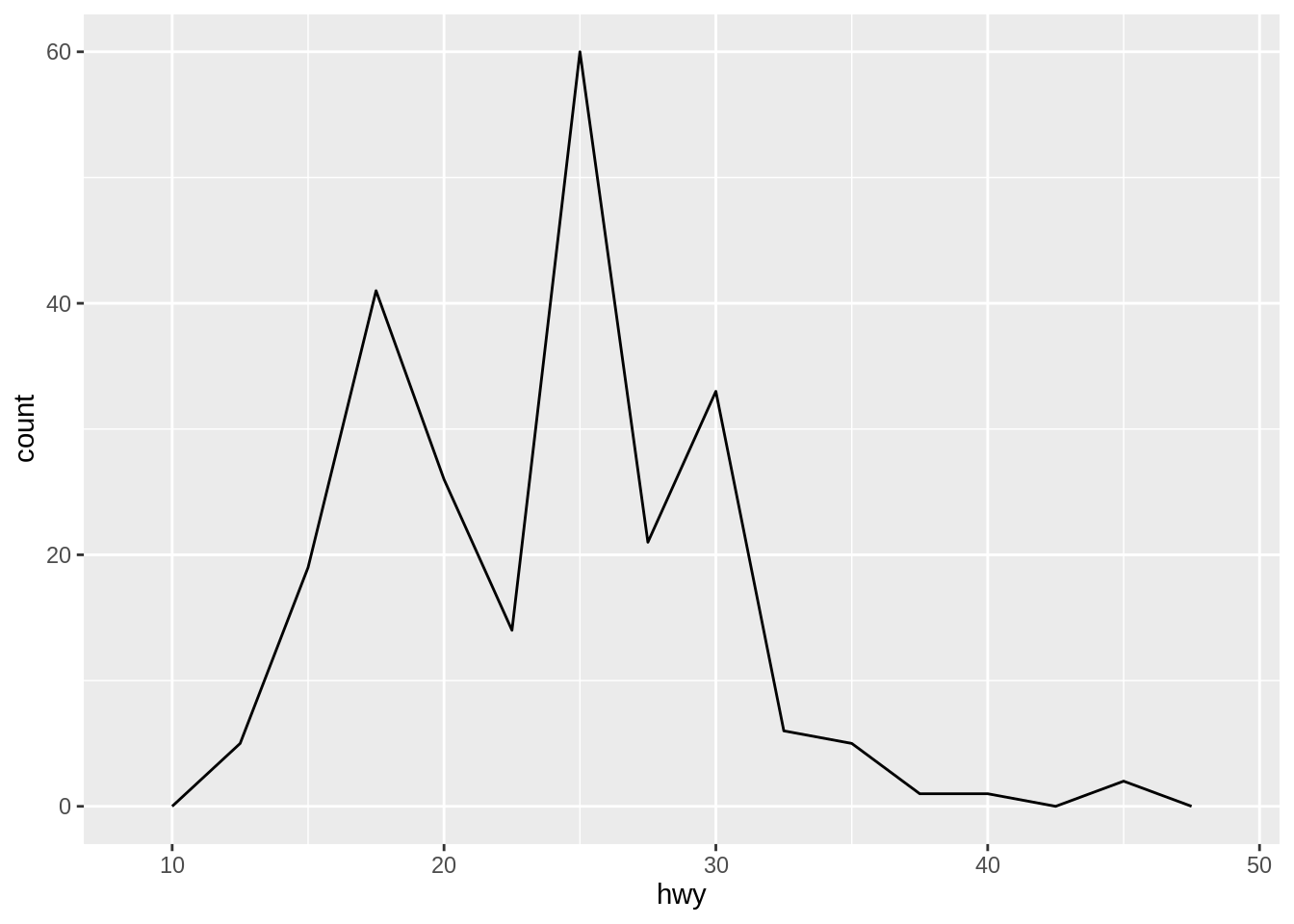
ggplot(mpg, aes(x = hwy)) + geom_histogram(binwidth = 2.5)

ggplot(mpg, aes(x = hwy)) + geom_freqpoly(binwidth = 2.5)

Like histogram, it is also important to specify the binwidth for geom_freqpoly().

An alternative to the frequency polygon is the density plot, geom_density(). It is sometimes nice to add the density curve on the histogram.

ggplot(mpg, aes(x = hwy)) + 
  geom_histogram(aes(y = after_stat(density)), 
                 binwidth = 2.5, alpha = 0.6) +
  geom_density(alpha = 0.5)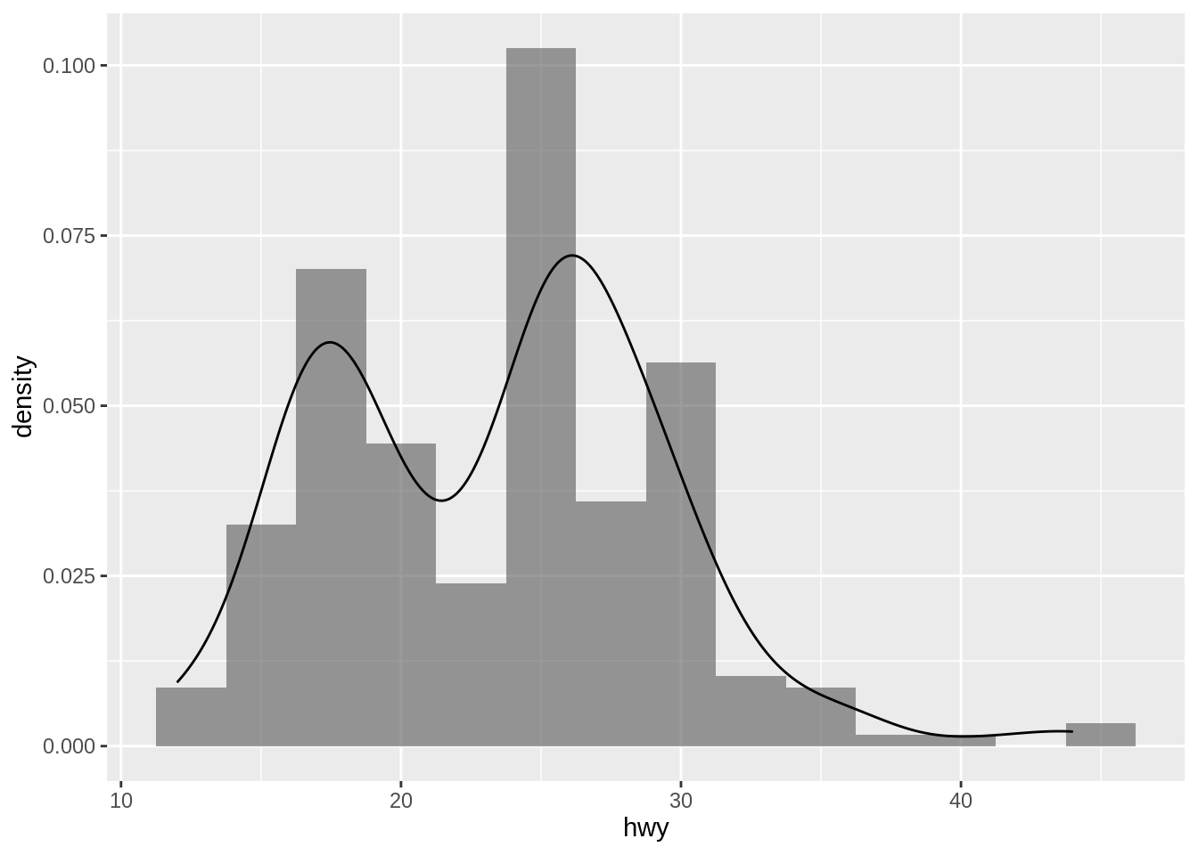

Note here that we need to specify the aesthetic of \(y\) in geom_histogram(). Otherwise, the y scales of the two graphs do not match.

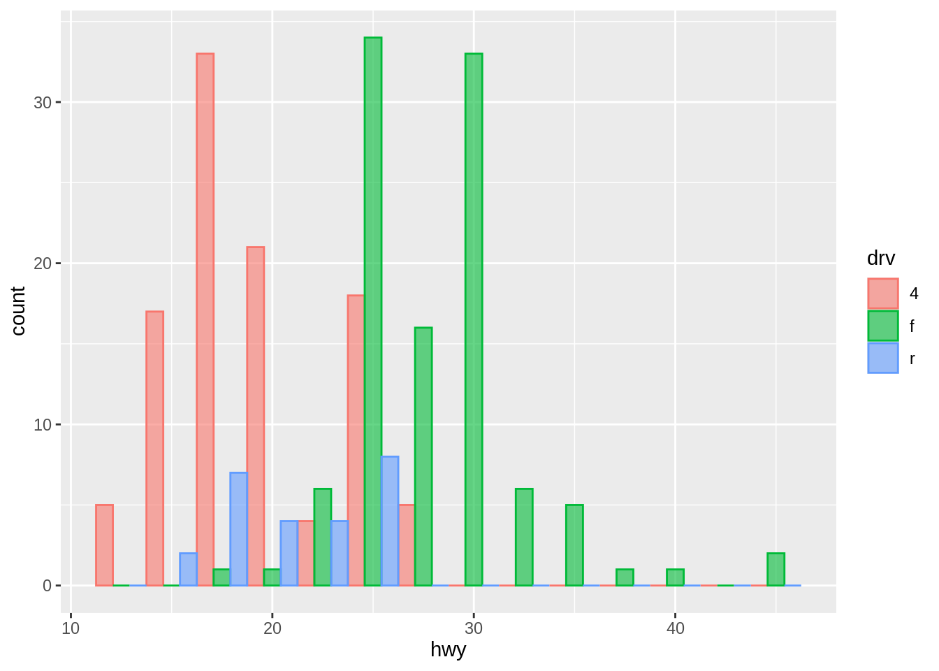
To compare the distributions of different subgroups, you can map a categorical variable to either fill (for geom_histogram()) or color (for geom_freqpoly()).

However, note that by default, the bars will be stacked in a histogram. If you want to compare the distributions side by side, you might consider setting the position argument to “dodge”.

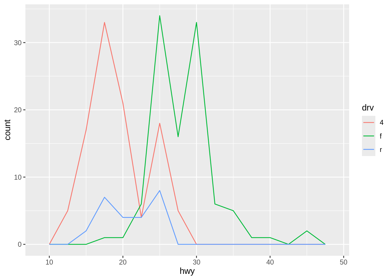
geom_freqpoly(), on the other hand, is more effective for comparing distributions as it overlays line plots of frequencies for each category. It can handle overlapping data better than histograms in some cases.

ggplot(mpg, aes(x = hwy, color = drv, fill = drv)) + 
  geom_histogram(binwidth = 2.5, alpha = 0.6, position = "dodge")

ggplot(mpg, aes(x = hwy, color = drv, fill = drv)) + 
  geom_freqpoly(binwidth = 2.5)

Exercise E

Work with the mpg data. Use faceting to create subplots so as to compare the distributions of displ for different drive trains drv. In each subplot, you can either use a histogram or a frequency polygon.

Work with the iris data. Draw a histogram to compare the distributions of Petal.Length for different Species. This time let us plot everything on one graph and add the density curves on top of the histograms.

library(tidyverse)