11 Data Manipulation Basics

Manipulation of data frames is a common task when you start exploring your data in R and dplyr is a package for making tabular data manipulation easier.

tidyverse is an “umbrella-package” that installs a series of packages useful for data analysis which work together well. Some of them are considered core packages (among them tidyr, dplyr, ggplot2), because you are likely to use them in almost every analysis. Other packages, like lubridate (to work with dates) or haven (for SPSS, Stata, and SAS data) that you are likely to use not for every analysis are also installed.

We can load the tidyverse package by calling

library(tidyverse)

Of course, if you have not installed this package yet, please do so by following my instructions in Lecture 1.

11.1 What is `dplyr`?

dplyr is one part of a larger tidyverse ecosystem that enables you to work with data in tidy data formats.

The package dplyr provides convenient tools for the most common data manipulation tasks. It is built to work directly with data frames, with many common tasks optimized by being written in a compiled language (C++). An additional feature is the ability to work directly with data stored in an external database. The benefits of doing this are that the data can be managed natively in a relational database, queries can be conducted on that database, and only the results of the query are returned.

To learn more about dplyr, you may want to check out the dplyr cheatsheet.

11.2 Grammar for data manipulation

The dplyr package presents a grammar for data wrangling with the ‘pipe’ operator |>. Hadley Wickham, one of the authors of dplyr, has identified five verbs for working with data in a data frame:

select() take a subset of the columns (i.e., features, variables)
filter() take a subset of the rows (i.e., observations)
mutate() add or modify existing columns
arrange() sort the rows
summarise() aggregate the data across rows (e.g., group it according to some criteria)

Each of these functions takes a data frame as its first argument, and returns a data frame. Thus, these five verbs can be used in conjunction with each other to provide a powerful means to slice-and-dice a single table of data. As with any grammar, what these verbs mean on their own is one thing, but being able to combine these verbs with nouns (i.e., data frames) creates an infinite space for data wrangling. Mastery of these five verbs can make the computation of most any descriptive statistic a breeze and facilitate further analysis. Wickham’s approach is inspired by his desire to blur the boundaries between R and the ubiquitous relational database querying syntax SQL.

11.3 Import data as tibbles

Recall from Lecture 3, when we used read_excel() to import the data, the loaded data appear as tibbles instead of the traditional R data frames. Here we will first explain a little about tibbles.

Exercise A

For illustration purposes, let us try to load an online sample data by calling the read_csv() function in the tidyverse package.

orderinfo <- read_csv("https://raw.githubusercontent.com/rsquaredacademy/datasets/master/web.csv")
head(orderinfo)

Tip

To assist your understanding of the data, below please find the description of the main variables in this data set:

referrer: referrer website/search engine
device: device used to visit the website
n_pages: number of pages visited
duration: time spent on the website (in seconds)
purchase: whether visitor purchased
order_value: order value of visitor (in dollars)
n_visit: number of visits

class(orderinfo)

[1] "spec_tbl_df" "tbl_df"      "tbl"         "data.frame"

You may have noticed that by using either read_excel() or read_csv(), we have generated an object of class tbl_df, also known as a “tibble”. Tibble’s data structure is very similar to a data frame. For our purposes the only differences are that

columns of class character are never converted into factors,
it tries to recognize and date types
the output displays the data type of each column under its name, and
it only prints the first few rows of data and only as many columns as fit on one screen. If we wanted to print all columns we can use the print command, and set the width parameter to Inf. To print the first 6 rows for example we would do this: print(my_tibble, n=6, width=Inf).

11.4 `select()` and `filter()`

To select columns of a data frame with dplyr, use select(). The first argument to this function is the data frame orderinfo, and the subsequent arguments are the columns to keep.

select(orderinfo, id, device, order_value)

We can select a set of columns using :. In the below example, we select all the columns starting from referrer up to order_items. Remember that we can use : only when the columns are adjacent to each other in the data set.

select(orderinfo, referrer:order_items)

What if you want to select all columns except a few? Typing the name of many columns can be cumbersome and may also result in spelling errors. We may use : only if the columns are adjacent to each other but that may not always be the case. dplyr allows us to specify columns that need not be selected using :. In the below example, we select all columns except n_pages and duration. Notice the - before both of them.

select(orderinfo, -n_pages, -duration)

Exercise B

Select the device and order_value columns from our orderinfo data set.

It is worth knowing that dplyr is backed by another package with a number of helper functions, which provide convenient functions to select columns based on their names. For example:

select(orderinfo, starts_with("order"))

Check out the tidyselect reference for more.

To subset rows based on specific criteria, we use filter():

filter(orderinfo, referrer == "direct")

We can specify multiple filtering conditions as well. In the below example, we specify two filter conditions:

“direct” referrer
resulted in a purchase or conversion

filter(orderinfo, referrer == "direct", purchase)

Exercise C

Select the rows by specifying the following conditions:

visit from device “tablet”
made a purchase
browsed less than 15 pages

11.5 `arrange()`

To sort rows by variables use the arrange() function:

arrange(orderinfo, device, n_pages)

If we want to arrange the data in descending order, we can use desc(). Let us arrange the data in descending order.

arrange(orderinfo, desc(n_pages))

Exercise D

Arrange orderinfo first by number of visits in ascending order and then by number of pages in a descending order.

11.6 `mutate()`

mutate()’s general syntax is detailed in the following figure.
Syntax for the mutate() function

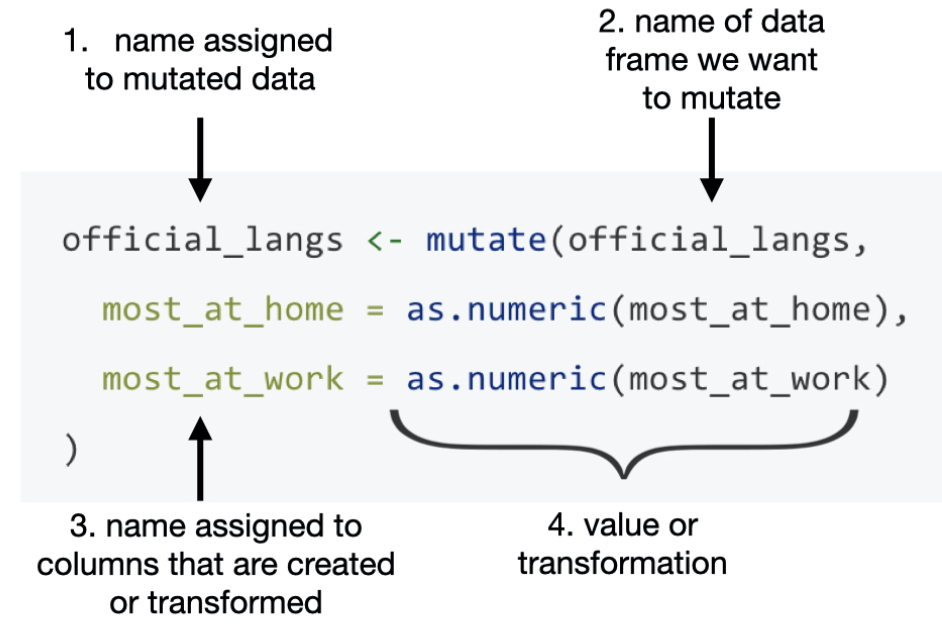
We can use the mutate() function to make modification on the current column. The following example is trying to change the data type of the device column to factor.

orderinfo_modified <- mutate(
  orderinfo, 
  device = as.factor(device)
  )

We can also use the mutate() function to create a new column based on the existing ones. For instance, we can calculate the average time spent per page by

mutate(orderinfo, avg_page_time = duration / n_pages)

Exercise E

Create a new column named avg_value in orderinfo which shows the average value per item purchased. Note that there will be many NaN (i.e., not a number) values in this column for the visits where no items were purchased.

11.7 `summarise()` with `group_by()`

Our last of the five verbs for single-table analysis is summarise(), which is nearly always used in conjunction with group_by(). The previous four verbs offer powerful and flexible ways to manipulate a data frame. However, the extent of the analysis we can perform with these verbs alone is limited. On the other hand, usingsummarise() with group_by() enables us to aggregate data effectively.

When used alone, summarise() collapses a data frame into a single row. Critically, we have to specify how we want to reduce an entire column of data into a single value. The method of aggregation that we specify controls what will appear in the output.

summarise(orderinfo, N = n(),
          min_duration = min(duration),
          num_google = sum(referrer == "google"),
          num_purchase = sum(purchase),
          mean_page = mean(n_pages)
          )

The function n() simply counts the number of rows. To help ensure that data aggregation is being done correctly, it is a good practice to use n() every time you use summarise().

It follows that we can also provide data aggregation by groups using group_by() and summarise() together.

# Step 1 - split data by referrer type
step1 <- group_by(orderinfo, referrer)
# Step 2 - compute average number of pages
step2 <- summarise(step1, mean(n_pages))
step2

Exercise F

Compute both the mean and median values for n_pages by referrer types.

11.8 Pipes

We have already seen before that we can combine the use of two functions group_by() and summarise(). We did it as a two-step process, which can clutter up your workspace with lots of objects.

Alternatively, you could try nested functions.

summarise(group_by(orderinfo, referrer), mean(n_pages))

This is handy, but can be difficult to read if too many functions are nested as things are evaluated from the inside out.

Now let us introduce a very nice grammar in tidyverse, i.e., the use of the pipe operator |>. Pipes let you take the output of one function and send it directly to the next, which is useful when you need to do many things to the same data set.

Tip

In this course, we will use the base R pipe operator, |>, inspired by the magrittr package’s %>% operator. Unlike %>%, which is part of the tidyverse metapackage via dplyr, the |> operator is built into R. While there are differences between the two, especially in advanced R applications like package development, these details are beyond our current scope. We mention %>% because it remains prevalent in data analysis and various data science resources. Generally, both operators are interchangeable in most analytical contexts.
In RStudio, you can type the native pipe |> using the keyboard shortcut Ctrl + Shift + M on a PC or Cmd + Shift + M on a Mac. However, ensure that the relevant option is enabled in the Global Options.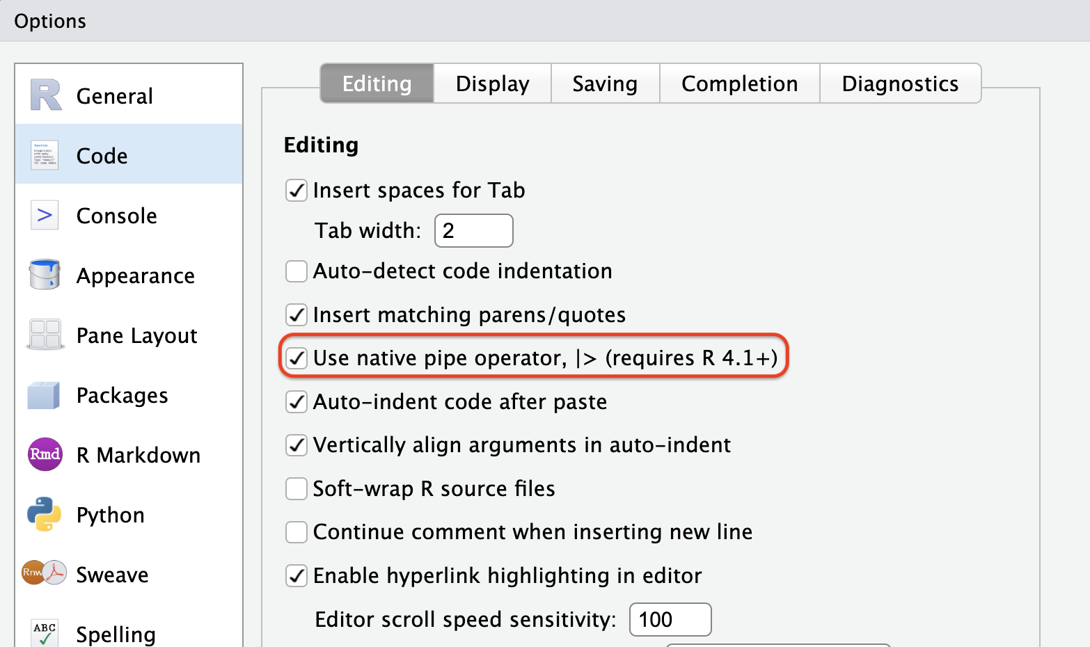

For instance, combine group_by() and summarise():

orderinfo |> 
  group_by(referrer) |> 
  summarise(N = n(), avg_page = mean(n_pages))

Another example: combine select() and filter():

orderinfo |>
  select(id, referrer, order_value) |> 
  filter(referrer == "direct")

Exercise G

Show a table presenting the average number of pages visited by purchasers and non-purchasers.