20  Output

library(tidyverse)

Most of the time you create a plot object and immediately render it, but you can also save a plot to a variable and manipulate it:

p <- ggplot(mpg, aes(x = displ, y = hwy, color = factor(cyl))) +
  geom_point()

Once you have a plot object, there are a few things you can do with it:

• Render it on screen by calling its name or with print(). This happens automatically when running interactively, but inside a loop or function, you’ll need to print() it yourself.

p

print(p)

• Save it to disk with ggsave().

# Save png to disk
ggsave("Output/plot.png", p, width = 5, height = 5)

• Briefly describe its structure with summary().

summary(p)

data: manufacturer, model, displ, year, cyl, trans, drv, cty, hwy, fl,
  class [234x11]
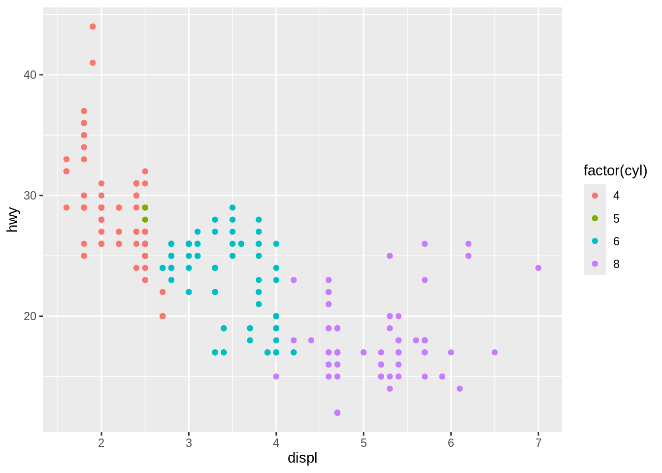
mapping:  x = ~displ, y = ~hwy, colour = ~factor(cyl)
faceting: <ggproto object: Class FacetNull, Facet, gg>
    compute_layout: function
    draw_back: function
    draw_front: function
    draw_labels: function
    draw_panels: function
    finish_data: function
    init_scales: function
    map_data: function
    params: list
    setup_data: function
    setup_params: function
    shrink: TRUE
    train_scales: function
    vars: function
    super:  <ggproto object: Class FacetNull, Facet, gg>
-----------------------------------
geom_point: na.rm = FALSE
stat_identity: na.rm = FALSE
position_identity 

• Save a cached copy of it to disk, with saveRDS(). This saves a complete copy of the plot object, so you can easily re-create it with readRDS().

saveRDS(p, "Output/plot.rds")
q <- readRDS("Output/plot.rds")

Exercise G

Q1

Save any of the graphs you have produced earlier to your local Output folder, assuming that you have a sub-folder called Output in our current working directory.