17 Faceting

Tip

flowchart LR
  AB{{Facet}}
  AB -->ABA(facet_wrap)
  AB -->ABB(facet_grid)
  classDef api fill:#f96,color:#fff

library(tidyverse)

Another technique for displaying additional categorical variables on a plot is faceting. Faceting creates tables of graphics by splitting the data into subsets and displaying the same graph for each subset.

There are two types of faceting: grid and wrapped. The differences between facet_wrap() and facet_grid() are illustrated below.

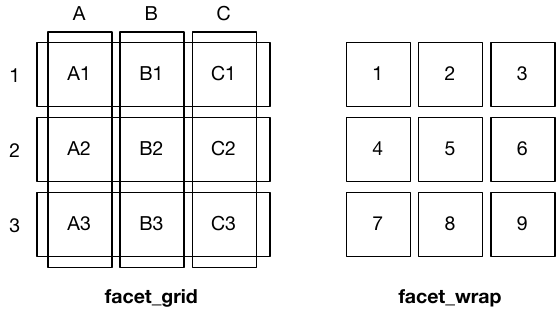
facet_grid() (left) is fundamentally 2d, being made up of two independent components. facet_wrap() (right) is 1d, but wrapped into 2d to save space.

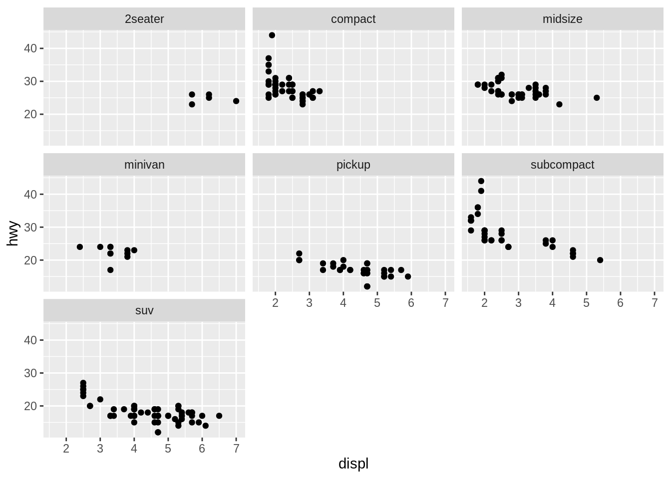
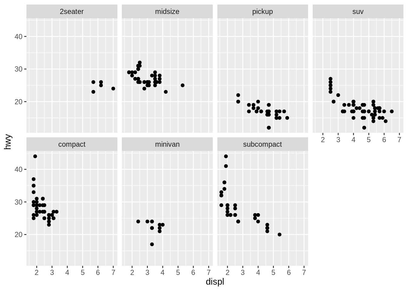
facet_wrap() makes a long ribbon of panels (generated by any number of variables) and wraps it into 2d. This is useful if you have a single variable with many levels and want to arrange the plots in a more space efficient manner. It takes the name of a variable preceded by ~.

ggplot(mpg, aes(x = displ, y = hwy)) + 
  geom_point() + 
  facet_wrap(~class)

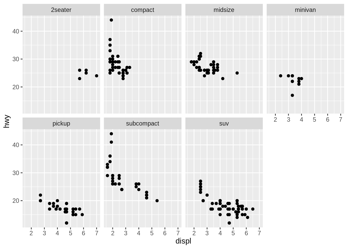
You can control how the ribbon is wrapped into a grid with ncol, nrow, as.table and dir.

ncol and nrow control how many columns and rows (you only need to set one).

ggplot(mpg, aes(x = displ, y = hwy)) + 
  geom_point() + 
  facet_wrap(~class, ncol = 4)

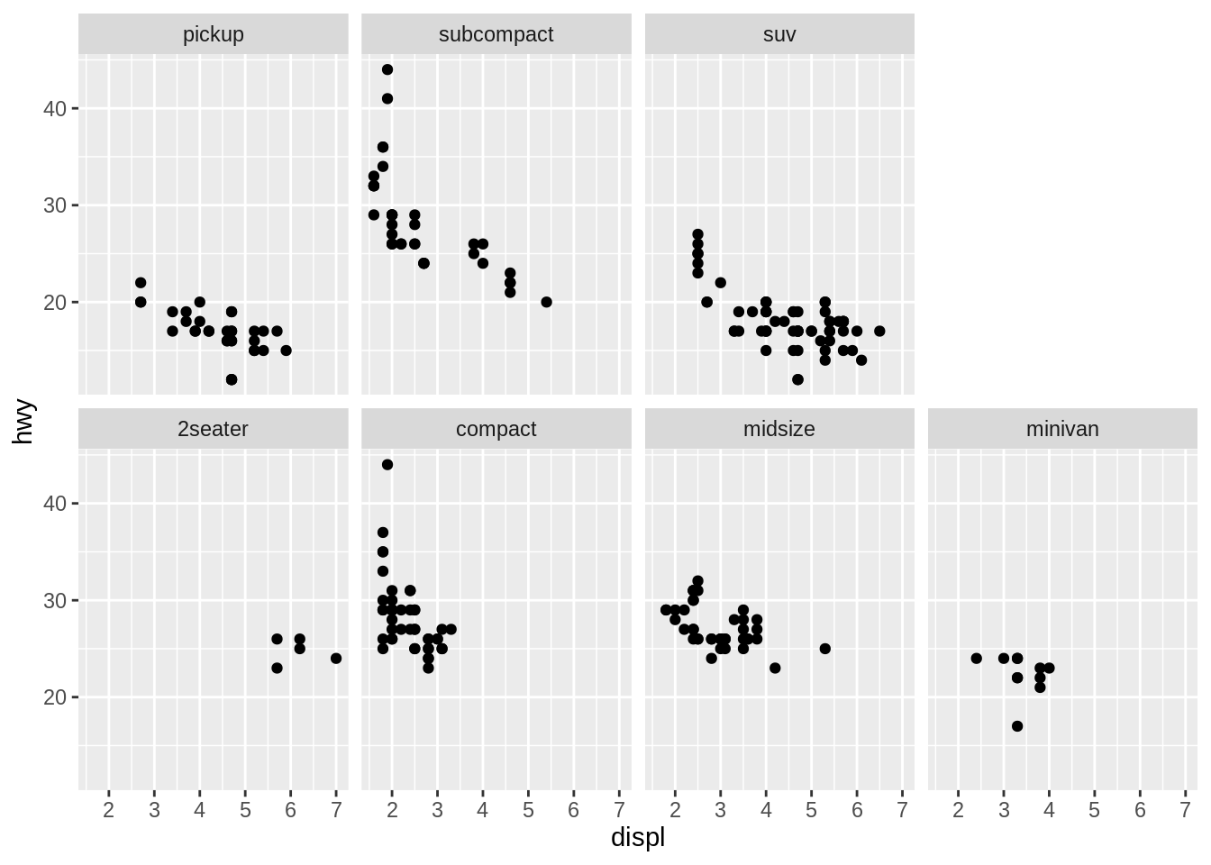
as.table controls whether the facets are laid out like a table (TRUE), with highest values at the bottom-right, or a plot (FALSE), with the highest values at the top-right.

ggplot(mpg, aes(x = displ, y = hwy)) + 
  geom_point() + 
  facet_wrap(~class, ncol = 4, as.table = F)

dir controls the direction of wrap: horizontal or vertical.

ggplot(mpg, aes(x = displ, y = hwy)) + 
  geom_point() + 
  facet_wrap(~class, ncol = 4, dir = "v")

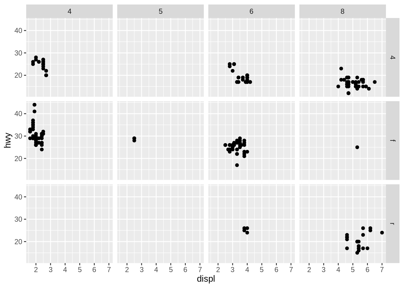
facet_grid() lays out plots in a 2d grid, as defined by a formula:

a ~ b spreads a across columns and b down rows. You’ll usually want to put the variable with the greatest number of levels in the columns, to take advantage of the aspect ratio of your screen.

ggplot(mpg, aes(x = displ, y = hwy)) + 
  geom_point() + 
  facet_grid(drv ~ cyl)

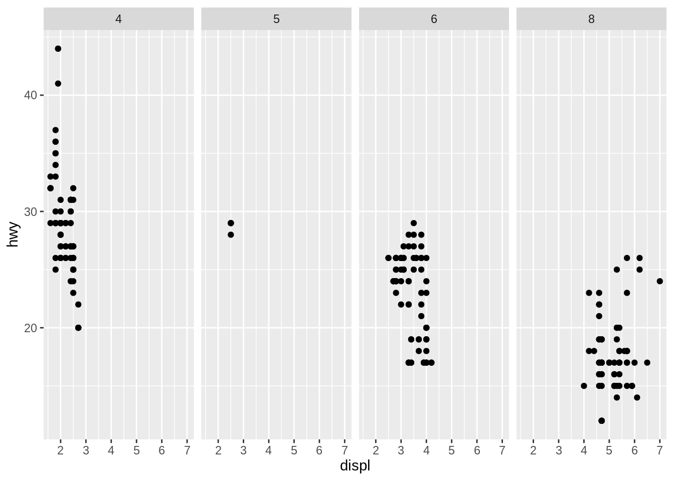
. ~ a spreads the values of a across the columns. This direction facilitates comparisons of \(y\) position, because the vertical scales are aligned.

ggplot(mpg, aes(x = displ, y = hwy)) + 
  geom_point() + 
  facet_grid(. ~ cyl)

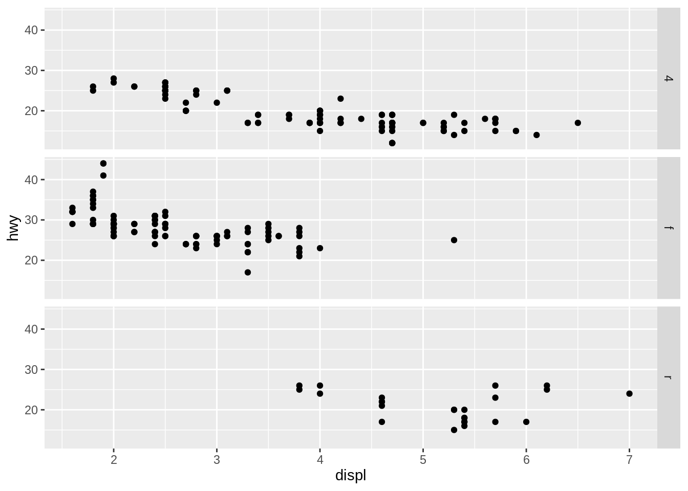
b ~ . spreads the values of b down the rows. This direction facilitates comparison of \(x\) position because the horizontal scales are aligned. This makes it particularly useful for comparing distributions.

ggplot(mpg, aes(x = displ, y = hwy)) + 
  geom_point() + 
  facet_grid(drv ~ .)

You can use multiple variables in the rows or columns, by “adding” them together, e.g. a + b ~ c + d. Variables appearing together on the rows or columns are nested in the sense that only combinations that appear in the data will appear in the plot. Variables that are specified on rows and columns will be crossed: all combinations will be shown, including those that didn’t appear in the original data set: this may result in empty panels.

Exercise C

What happens if you try to facet by a continuous variable like cty?

Use faceting to explore the cross-sectional (year year, and fuel type fl) relationship between city fuel economy cty, engine size displ. How does faceting by fuel type and year change your assessment of the relationship between engine size and fuel economy?