15 Introduction to Data Visualization
Like descriptive statistics, the purpose of a visualization is to answer a question about a data set of interest. So naturally, the first thing to do before creating a visualization is to formulate the question about the data you are trying to answer. A good visualization will clearly answer your question without distraction; a great visualization will suggest even what the question was itself without additional explanation. Imagine your visualization as part of a poster presentation for a project; even if you aren’t standing at the poster explaining things, an effective visualization will convey your message to the audience.
With the visualizations we will cover in this chapter, we will again focus on addressing descriptive and exploratory questions. Be careful to not answer any predictive, inferential, causal or mechanistic questions with the visualizations presented here, as we have not learned the tools necessary to do that properly just yet.
As with most coding tasks, it is totally fine (and quite common) to make mistakes and iterate a few times before you find the right visualization for your data and question.
Graphics is a great strength of R. The graphics package is part of the standard distribution and contains many useful functions for creating a variety of graphic displays. The base functionality has been expanded and made easier with ggplot2, part of the tidyverse of packages. In this module, we will focus on examples using ggplot2, and we will occasionally suggest other packages.
As usual, let us first load the tidyverse package by calling
15.1 ggplot2 basics
While the package is called ggplot2, the primary plotting function in the package is called ggplot. It is important to understand the basic pieces of a ggplot2 graph. Let us see a simple example:
In the preceding example, you can see that we pass data into ggplot, then define how the graph is created by stacking together small phrases that describe some aspect of the plot. This stacking together of phrases is part of the “grammar of graphics” ethos (that’s where the gg comes from). To learn more, you can read “A Layered Grammar of Graphics” written by ggplot2 author Hadley Wickham. The “grammar of graphics” concept originated with Leland Wilkinson, who articulated the idea of building graphics up from a set of primitives (i.e., verbs and nouns).
As we talk about ggplot graphics, it’s worth defining the components of a ggplot graph:
aesthetics
The aesthetics, or aesthetic mappings, communicate toggplotwhich fields in the source data get mapped to which visual elements in the graphic. This is theaesline in aggplotcall.geometric object functions
These are geometric objects that describe the type of graph being created. These start withgeom_and examples includegeom_line,geom_boxplot, andgeom_point, along with dozens more.layer
A layer is a combination of data, aesthetics, a geometric object, a stat, and other options to produce a visual layer in the ggplot graphic.facet functions
Facets are subplots where each small plot represents a subgroup of the data. The faceting functions includefacet_wrapandfacet_grid.stats
Stats are statistical transformations that are done before displaying the data. Not all graphs will have stats, but a few common stats arestat_ecdf(the empirical cumulative distribution function) andstat_identity, which tellsggplotto pass the data without doing any stats at all.themes
Themes are the visual elements of the plot that are not tied to data. These might include titles, margins, legend locations, or font choices.
ggplot
One of the first sources of confusion for new ggplot users is that they are inclined to reshape their data to be “wide” before plotting it. “Wide” here means every variable they are plotting is its own column in the underlying data frame. This is an approach that many users develop while using Excel and then bring with them to R. ggplot works most easily with “long” data where additional variables are added as rows in the data frame rather than columns. The great side effect of adding more measurements as rows is that any properly constructed ggplot graphs will automatically update to reflect the new data without changing the ggplot code. If each additional variable were added as a column, then the plotting code would have to be changed to introduce additional variables. This idea of “long” versus “wide” data will become more obvious in the examples in the rest of this module.
15.2 Creating a Scatter Plot
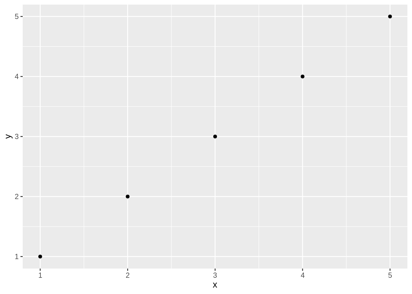
A scatter plot is used when you have paired observations: \((x_1, y_1), (x_2, y_2), \ldots, (x_n, y_n)\). It’s associated with a question: Is there a relationship between X and Y? We can plot the data by calling ggplot, passing in the data frame, and invoking a geometric point function:
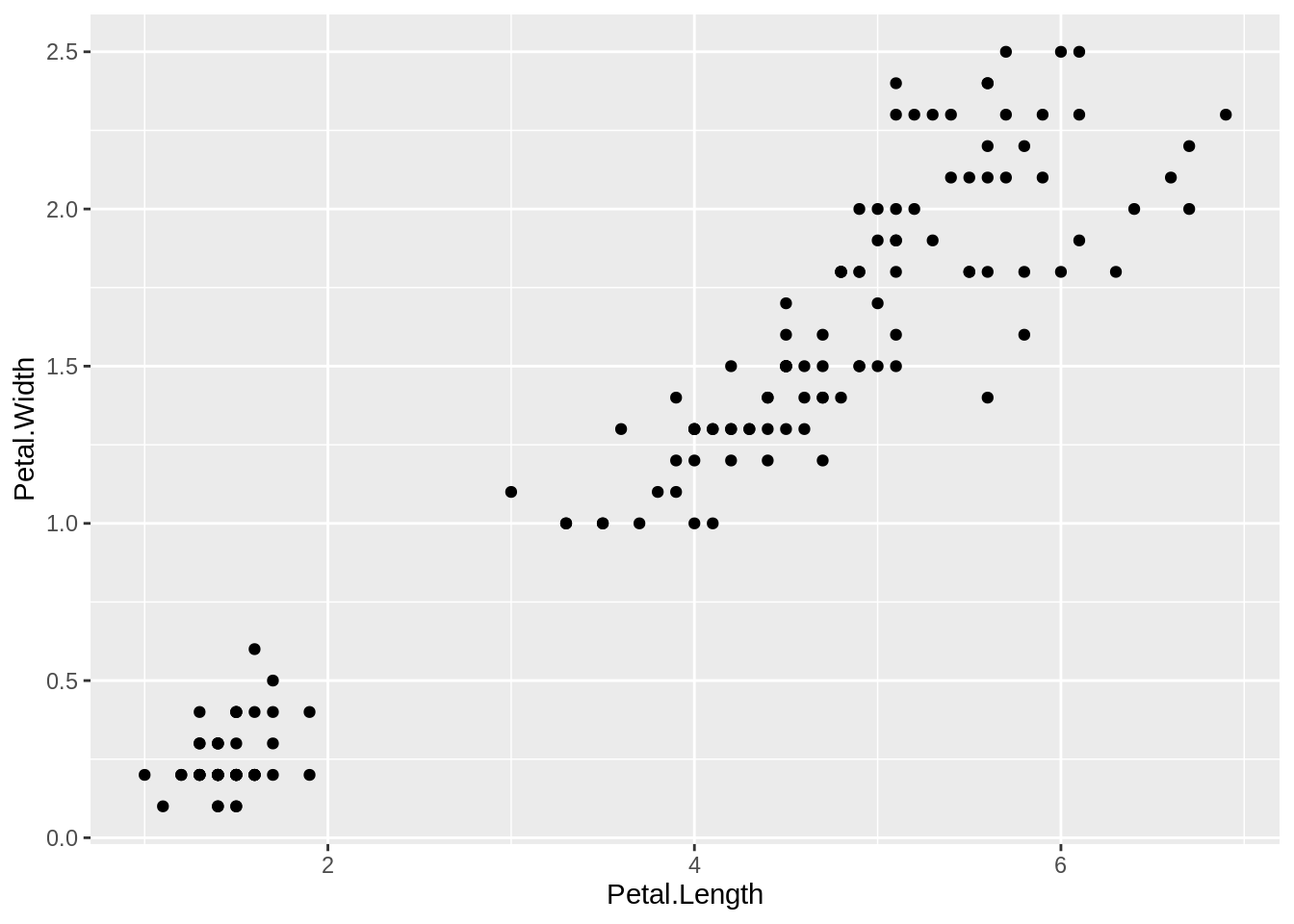
A scatter plot is a common first attack on a new dataset. It’s a quick way to see the relationship, if any, between \(x\) and \(y\).
Plotting with ggplot requires telling ggplot what data frame to use, then what type of graph to create, and which aesthetic mapping (aes) to use. The aes in this case defines which field from iris goes into which axis on the plot. Then the command geom_point communicates that you want a point graph, as opposed to a line or other type of graphic.
Exercise A
15.3 Creating a Line Plot
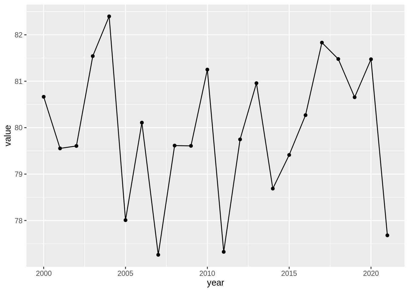
Line plots are used to visualize trends with respect to an independent, ordered quantity (e.g. time). A typical question could be: Does the X change over time, and are there any interesting patterns to note?
data_ex2 <- data.frame(year = seq(2000, 2021),
                       value = rnorm(22, mean = 80, sd = 2)) # generate 22 random values from a normal distribution
ggplot(data_ex2, aes(x = year, y = value)) +
  geom_line()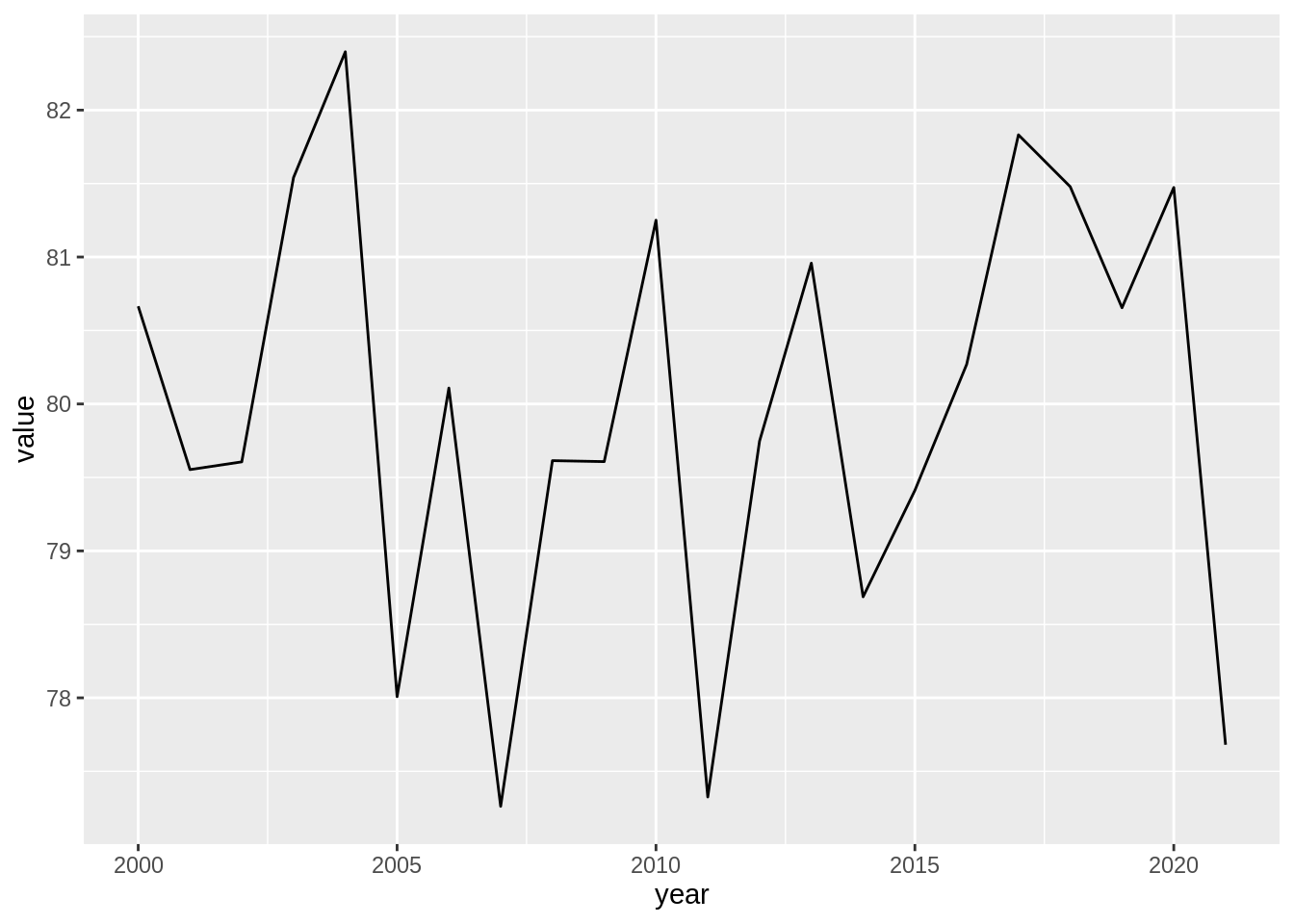
You can also add points using geom_point().
Note it’s common with ggplot to split the command on multiple lines, ending each line with a + so that R knows that the command will continue on the next line.
Exercise B
Work with the Weekly data from the ISLR package.
15.4 Creating a Bar Plot
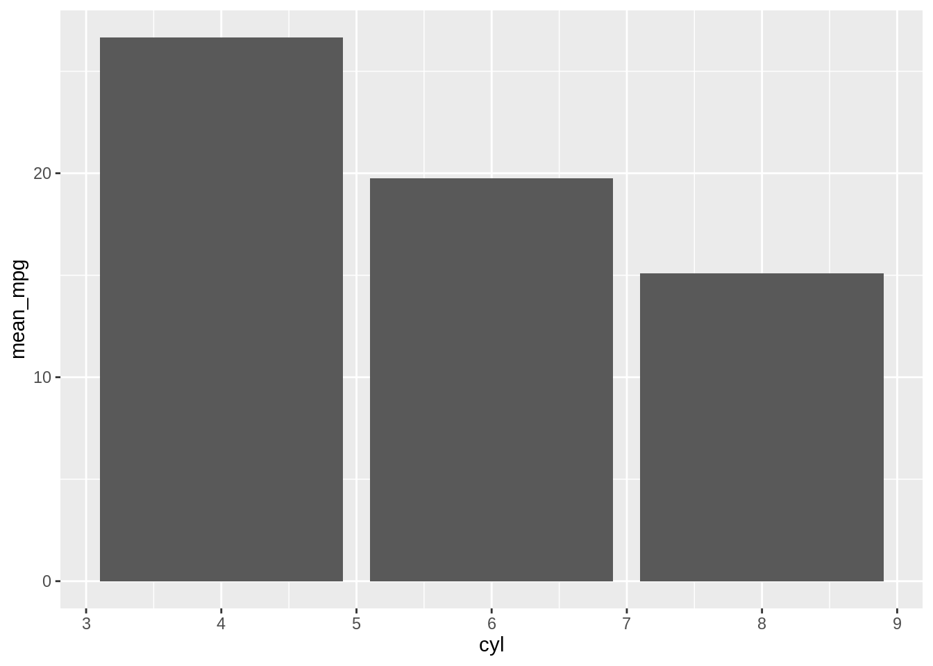
Bar plots are good for visualizing comparisons of amounts. A typical question can be something like: Do cars with more cylinders have lower miles per gallon? Hence, we can make a bar plot of the average miles per gallon by number of cylinders, we first create a data frame containing the mean values.
Then with ggplot2 we can use geom_col(). Notice the difference in the output when the \(x\) variable is continuous and when it is discrete:
# Bar plot of values. This uses the avg_mpg data frame, with the
# "cyl" column for x values and the "mean_mpg" column for y values.
ggplot(avg_mpg, aes(x = cyl, y = mean_mpg)) +
  geom_col()
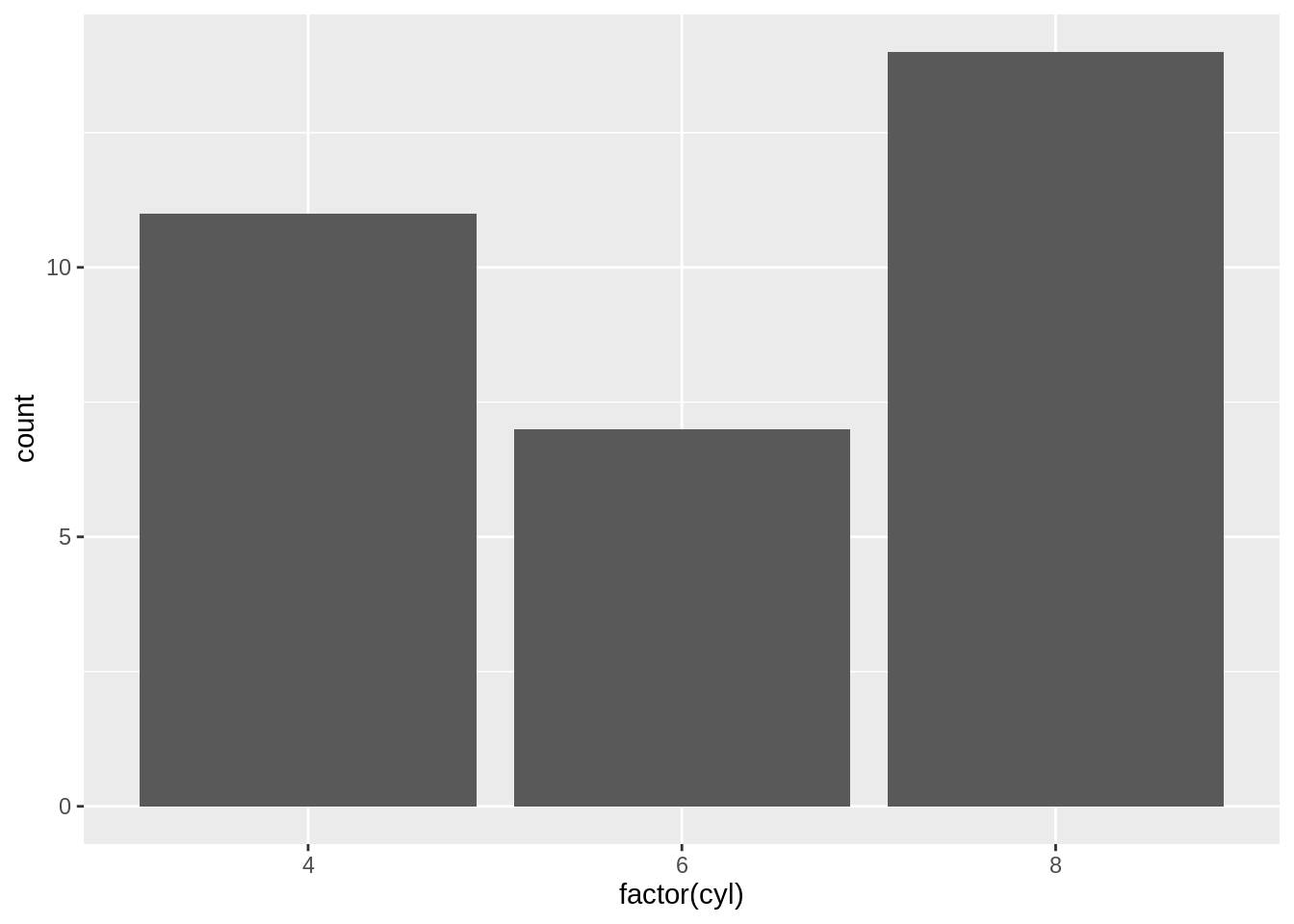
# Convert the x variable to a factor, so that it is treated as discrete
ggplot(avg_mpg, aes(x = factor(cyl), y = mean_mpg)) +
  geom_col()
ggplot2 can also be used to plot the count of the number of data rows in each category, by using geom_bar() instead of geom_col(). Once again, notice the difference between a continuous \(x\)-axis and a discrete one. For some kinds of data, it may make more sense to convert the continuous \(x\) variable to a discrete one, with the factor() function.
# Bar plot of counts. This uses the mtcars data frame, with the
# "cyl" column for x position. The y position is calculated by
# counting the number of rows for each value of cyl.
ggplot(mtcars, aes(x = cyl)) +
  geom_bar()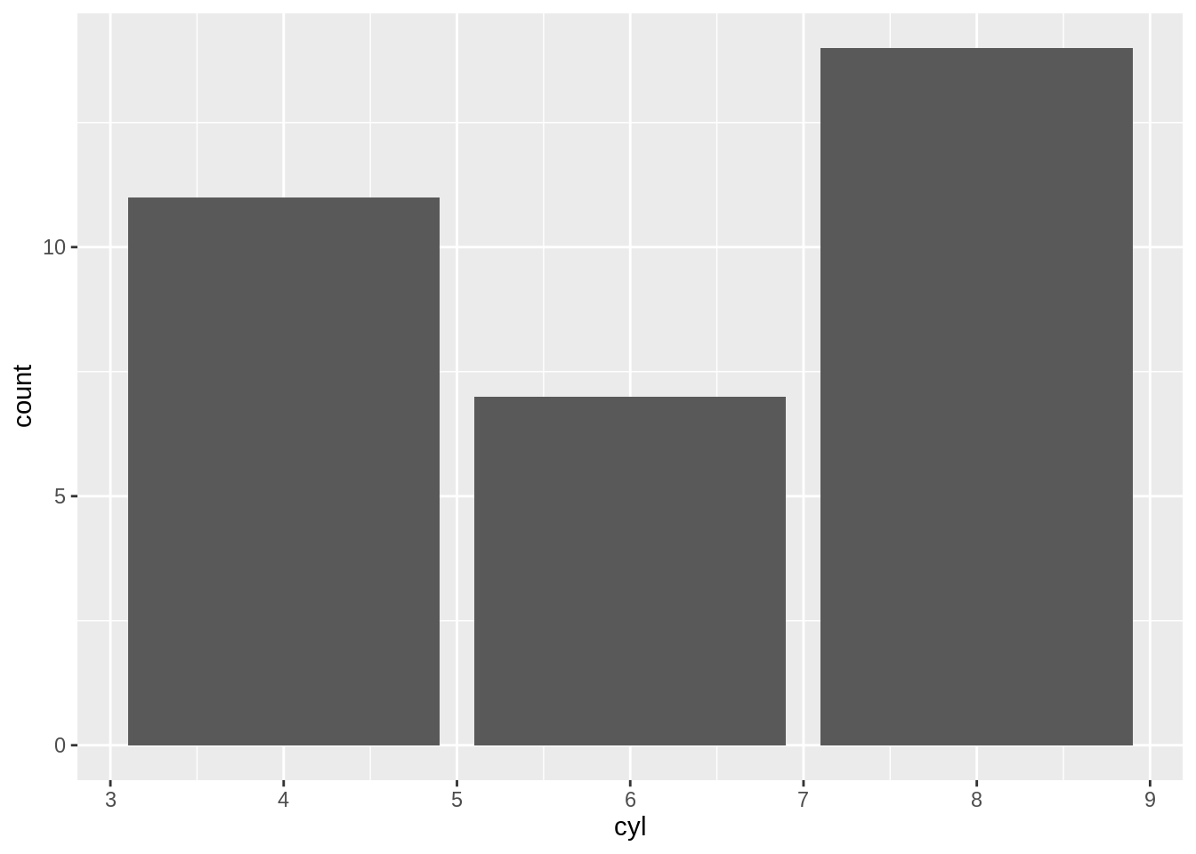
Exercise C
Alternatively, you can use geom_bar() to create the bar chart with the y-axis displaying mean_mpg, but you will need to set additional arguments in the geom_bar() function.
By default, geom_bar() uses the stat = “count” argument, which automatically counts the number of observations in each category of a factor.
geom_col() is essentially a shortcut for geom_bar(stat = "identity"), where it directly takes the y-values provided without performing any statistical transformation.
While geom_bar() and geom_col() can be used to achieve similar visual outcomes, their default functionalities cater to different types of data input - raw and summarized data, respectively.
15.5 Creating a Histogram
Histograms are used to visualize the distribution of a quantitative variable, i.e., all its possible values and how often they occur over different intervals. It is associated with the question: what is a typical value for miles per gallon? What’s the range of it?
With the ggplot2, you can produce a histogram using geom_histogram().
`stat_bin()` using `bins = 30`. Pick better value with `binwidth`.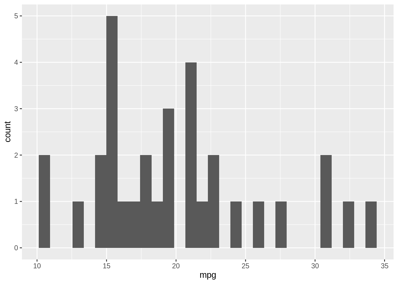
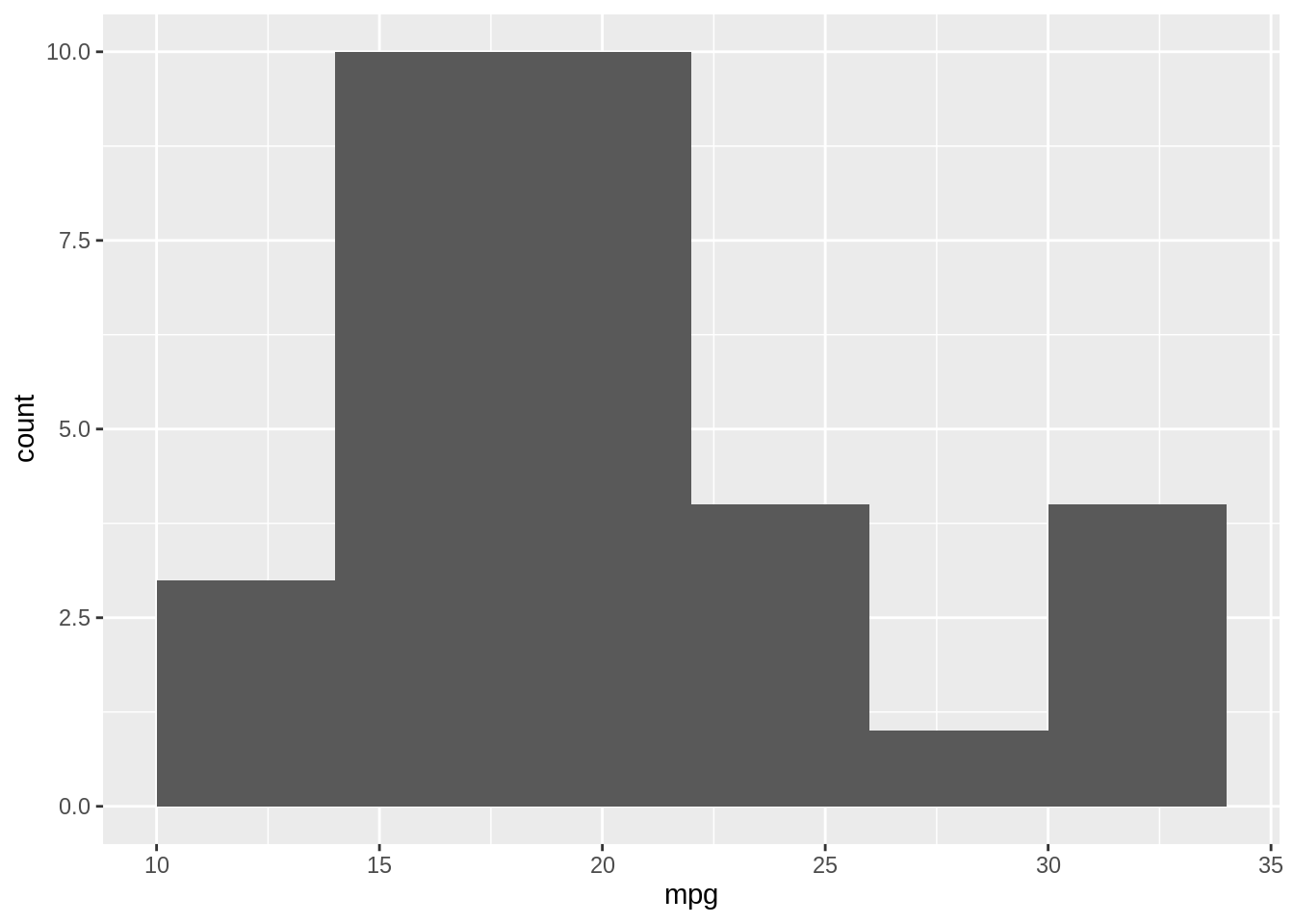
When you create a histogram without specifying the bin width, ggplot() prints out a message telling you that it’s defaulting to 30 bins, and to pick a better bin width. This is because it’s important to explore your data using different bin widths; the default of 30 bins may or may not show you something useful about your data. Now let us try a wider bin width which corresponds to smaller number of bins.
Exercise D
15.6 Creating a Boxplot
Boxplots are another tool for visualizing data distributions, so you can use them to answer similar questions from above. The following diagram depicts how a histogram and a box plot is created. 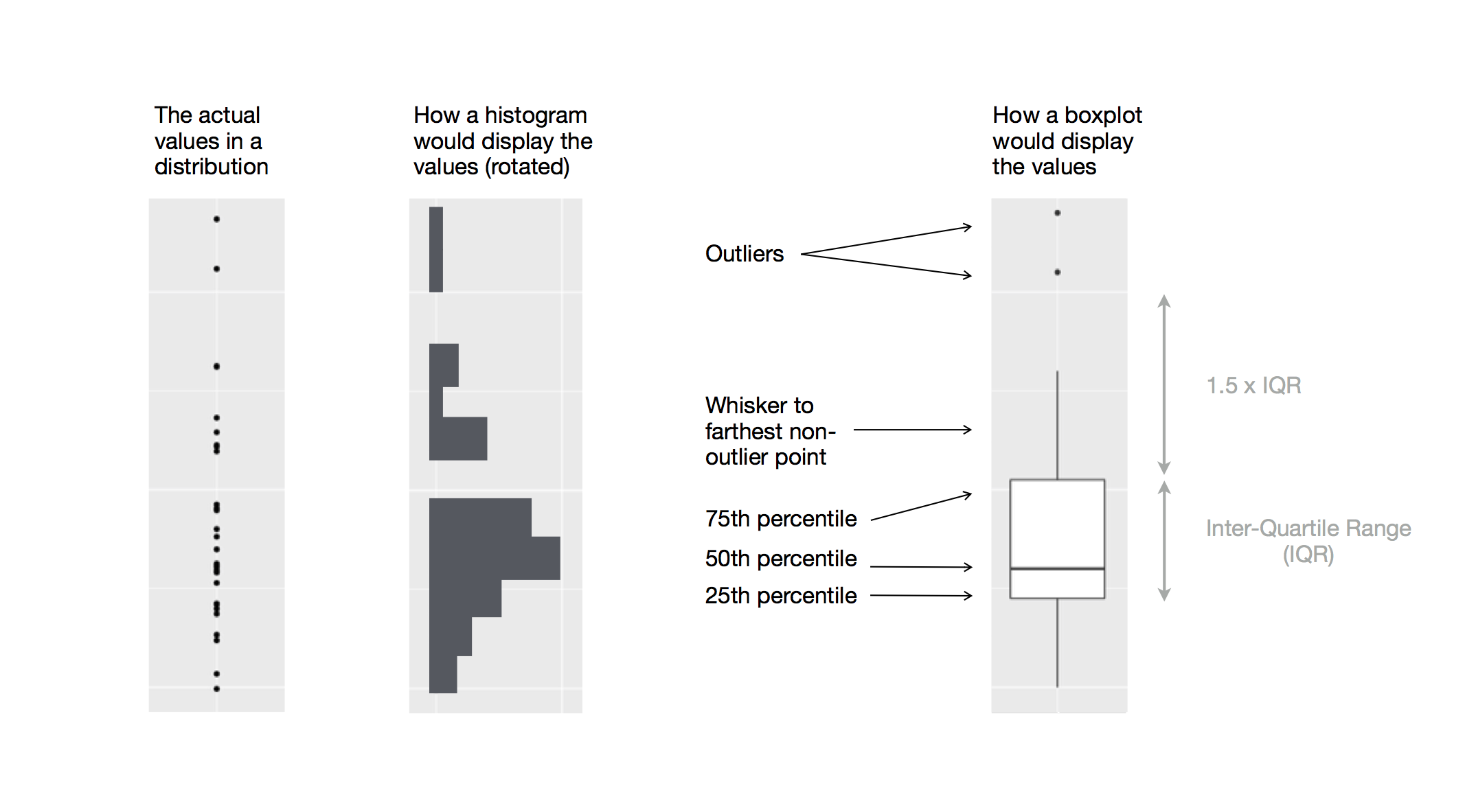
A boxplot directly displays summary statistics including first quartile, median, and third quartile. The upper whisker extends from the hinge to the largest value no further than 1.5 * IQR from the hinge (where IQR is the inter-quartile range, or distance between the first and third quartiles). The lower whisker extends from the hinge to the smallest value at most 1.5 * IQR of the hinge. Data beyond the end of the whiskers are called “outlying” points and are plotted individually. Boxplots are especially useful when comparing distributions across different categories or groups side by side.
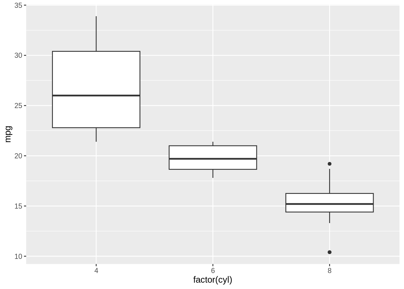
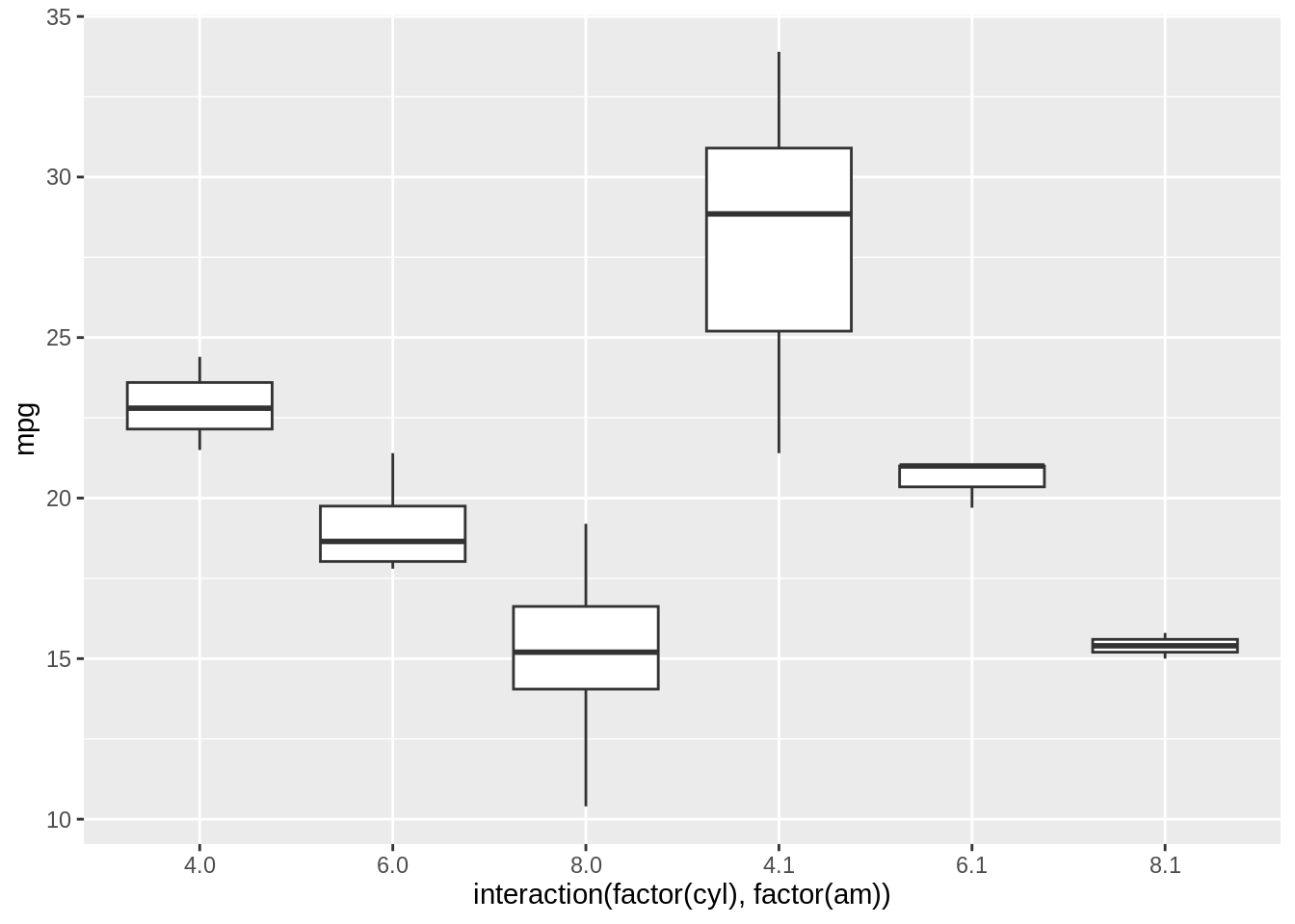
It’s also possible to make box plots for a combination of two grouping variables, with the interaction() function: