flowchart TD
  A((dplyr)) -->|two datasets|AD{{join}}
  AD --> ADA{{mutating}}
  ADA --> ADAA(inner):::api
  ADA --> ADAB(outer):::api
  ADA --> ADAC(left):::api
  ADA --> ADAD(right):::api
  ADA --> ADAE(full):::api
  AD --> ADB{{filtering}}
  ADB --> ADBA(semi):::api
  ADB --> ADBB(anti):::api
  classDef api fill:#f96,color:#fff
12 Join data using dplyr
Previously, we focused on the five-verb functions in dplyr and got familiar with the pipe operator. Here, we will continue to explore a few more functions and discover what else we can do with dplyr.
It is rare that a data analysis involves only a single table of data. Typically you have many tables of data, and you must combine them to answer the questions that you’re interested in. This section will first introduce you to two important types of joins:
- Mutating joins, which add new variables to one data frame from matching observations in another.
- Filtering joins, which filter observations from one data frame based on whether or not they match an observation in another.
We’ll begin by discussing keys, the variables used to connect a pair of data frames in a join. We cement the theory with an examination of the keys in two simple data sets, then use that knowledge to start joining data frames together.
Let us load the tidyverse package first.
In this section, we will be working on two data sets. The first one, order, contains details of orders placed by different customers. The second data set, customer contains details of each customer. The lists below demonstrate the variables in each data set.
order
- customer_id
- order_date
- amount
customer
- customer_id
- first_name
- city
Let us import both the data sets using read_delim which allows us to read in files with any delimiter.
order <- read_delim('https://raw.githubusercontent.com/rsquaredacademy/datasets/master/order.csv', delim = ';')
order
customer <- read_delim('https://raw.githubusercontent.com/rsquaredacademy/datasets/master/customer.csv', delim = ';')
customer12.1 Keys
Every join involves a pair of keys: a primary key and a foreign key. A primary key is a variable or set of variables that uniquely identifies each observation. When more than one variable is needed, the key is called a compound key. For example, customer records three pieces of data about each order: customer id, first name, and state where their city is in. You can identify a customer with the id, making id the primary key.
Exercise A
A foreign key is a variable (or set of variables) that corresponds to a primary key in another table. For example: order$id is a foreign key that corresponds to the primary key customer$id.
Now that that we’ve identified the primary keys in each table, it’s good practice to verify that they do indeed uniquely identify each observation. One way to do that is to count() the primary keys and look for entries where n is greater than one. This reveals that customer looks good:
You should also check for missing values in your primary keys - if a value is missing then it can’t identify an observation!
Exercise B
To do join data sets, we will need to use the family of *_join() functions provided in dplyr.
inner_joinleft_joinright_joinfull_joinsemi_joinanti_join
They all have the same interface: they take a pair of data frames (\(x\) and \(y\)) and return a data frame. The order of the rows and columns in the output is primarily determined by \(x\).
12.2 Mutating joins
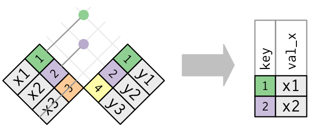
12.2.1 Inner join
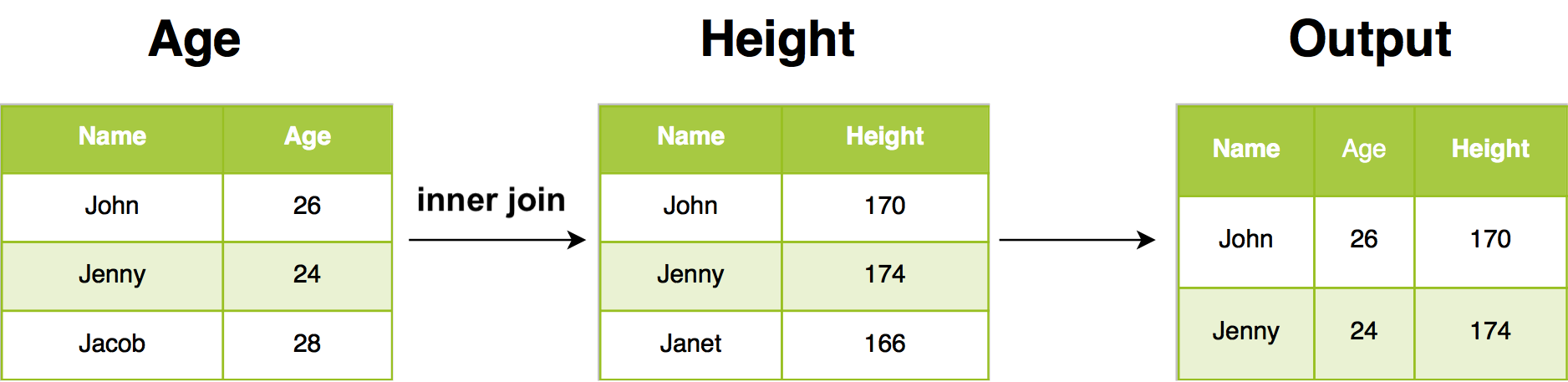
The simplest type of join is the inner join. An inner join matches pairs of observations whenever their keys are equal. The most important property of an inner join is that unmatched rows are not included in the result. This means that generally inner joins are usually not appropriate for use in analysis because it’s too easy to lose observations.
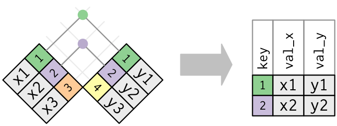
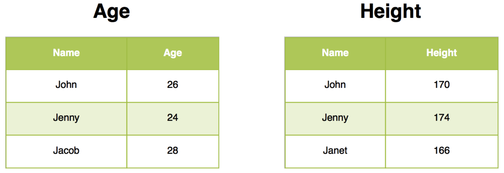
We will use two sample data sets to illustrate how inner join works. You can view the example data sets below.
Inner join will return all rows from Age where there are matching values in Height, and all columns from Age and Height. If there are multiple matches between Age and Height, all combination of the matches are returned.
Exercise C
12.2.2 Outer joins
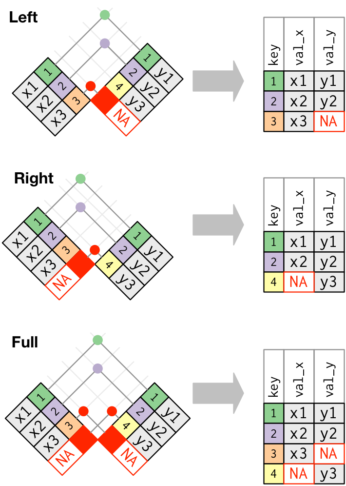
An inner join keeps observations that appear in both tables. An outer join keeps observations that appear in at least one of the tables. There are three types of outer joins:
- A left join keeps all observations in
x. - A right join keeps all observations in
y. - A full join keeps all observations in
xandy.
These joins work by adding an additional “virtual” observation to each table. This observation has a key that always matches (if no other key matches), and a value filled with NA. Graphically, that looks like:
The most commonly used join is the left join: you use this whenever you look up additional data from another table, because it preserves the original observations even when there isn’t a match. The left join should be your default join: use it unless you have a strong reason to prefer one of the others.
Another way to depict the different types of joins is with a Venn diagram:
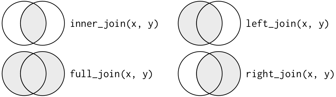
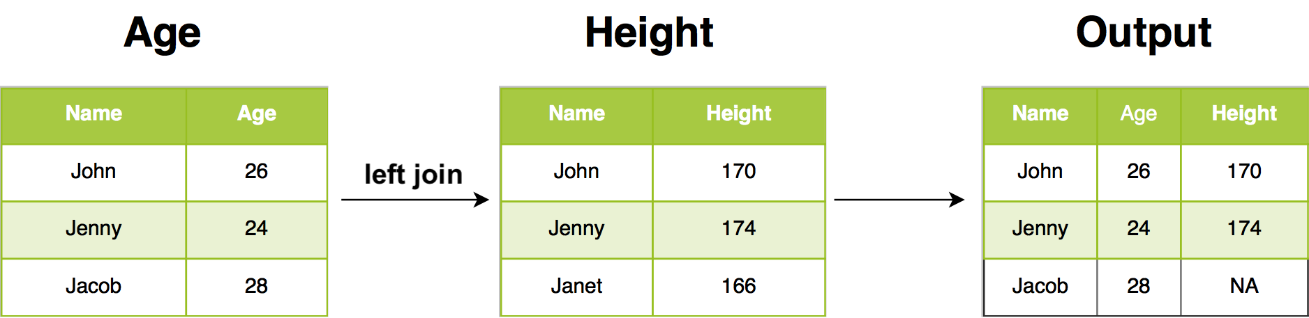
12.2.3 Left join
In our example, left join return all rows from Age, and all columns from Age and Height. Rows in Age with no match in Height will have NA in the new columns. If there are multiple matches between Age and Height, all combinations of the matches are returned.
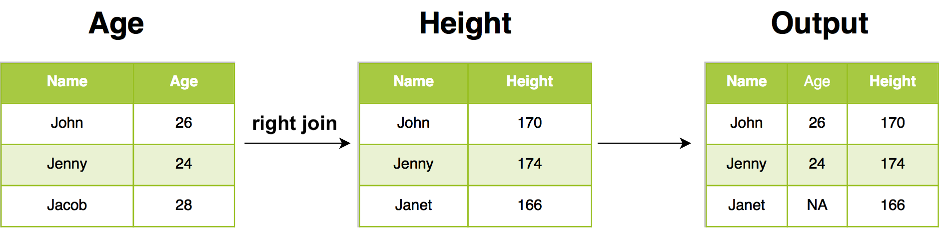
12.2.4 Right join
In our example, right join return all rows from Height, and all columns from Age and Height. Rows in Height with no match in Age will have NA in the new columns. If there are multiple matches between Age and Height, all combinations of the matches are returned.
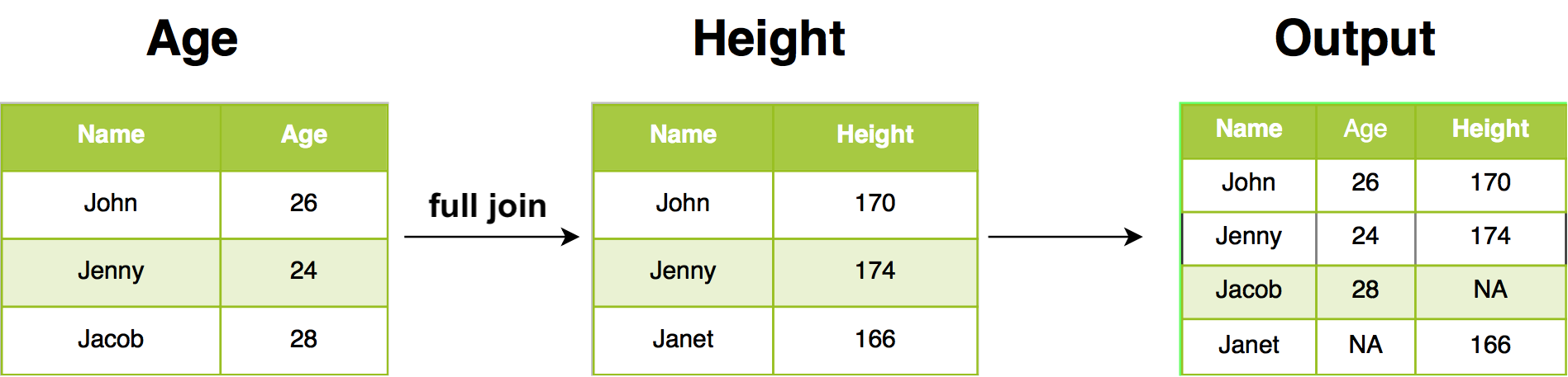
12.2.5 Full join
Full join return all rows and all columns from both Age and Height. Where there are not matching values, returns NA for the one missing.
Exercise D
Working with our order and customer data, first indicate the *_join() function that should be used for each of the following tasks and then implement them in your own R session.
12.3 Filtering joins
Filtering joins match observations in the same way as mutating joins, i.e., inner and outer joins, but affect the observations, not the variables. There are two types:
semi_join(x, y)keeps all observations inxthat have a match iny.anti_join(x, y)drops all observations inxthat have a match iny.
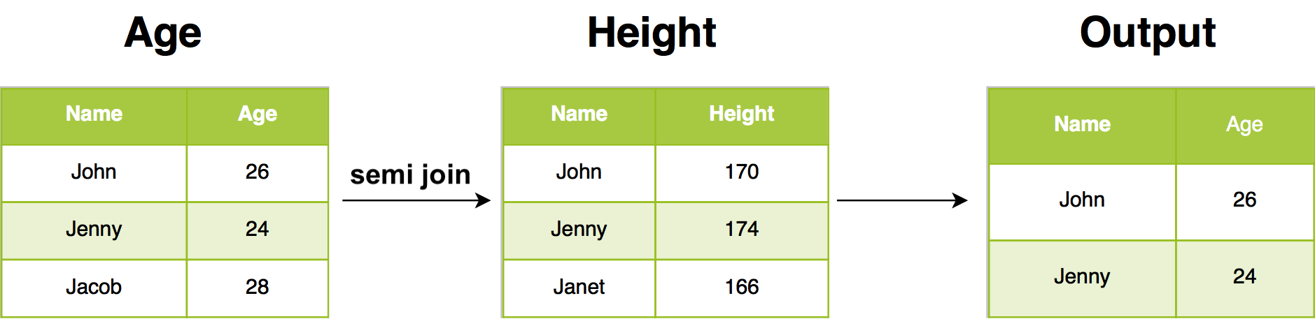
12.3.1 Semi join
Semi join connects the two tables like a mutating join, but instead of adding new columns, only keeps the rows in x that have a match in y:
Only the existence of a match is important; it doesn’t matter which observation is matched. This means that filtering joins never duplicate rows like mutating joins do:
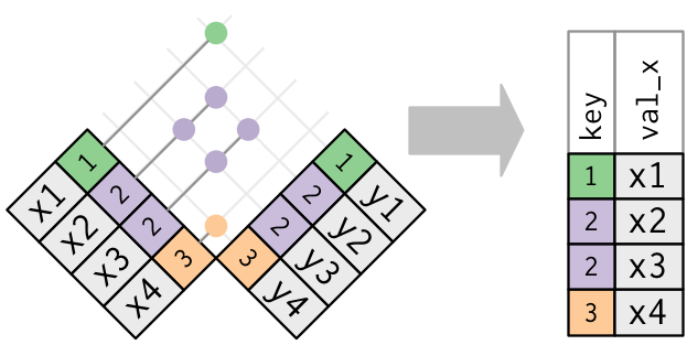
For example, semi join return all rows from Age where there are matching values in Height, keeping just columns from Age. A semi join differs from an inner join because an inner join will return one row of Age for each matching row of Height, where a semi join will never duplicate rows of Age.
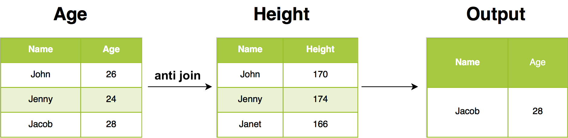
12.3.2 Anti join
The inverse of a semi join is an anti join. An anti join keeps the rows that don’t have a match:
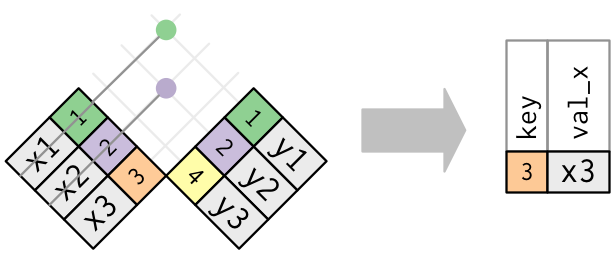
Anti joins are useful for diagnosing join mismatches. In our example, anti join return all rows from Age where there are not matching values in Height, keeping just columns from Age.
Exercise E
Working with our order and customer data, first indicate the *_join() function that should be used for each of the following tasks and then implement them in your own R session.