26 Machine Learning

26.1 Data Pre-processing

This step focuses on making data suitable for modeling by using data transformations. All transformations can be accomplished with dplyr, or other tidyverse packages. Consider using tidymodels packages when model development is more heavy and complex.

We will use the ISLR::Default dataset for illustration purposes. Once you load the ISLR package, its data is already imported and sufficiently tidy for immediate use in modeling.

library(ISLR)
Default

Apart from loading its core modeling packages, tidymodels also conveniently loads some tidyverse packages, including dplyr, tidyr and ggplot2.

library(tidymodels)

── Attaching packages ────────────────────────────────────── tidymodels 1.2.0 ──

✔ broom        1.0.7     ✔ recipes      1.1.0
✔ dials        1.3.0     ✔ rsample      1.2.1
✔ dplyr        1.1.4     ✔ tibble       3.2.1
✔ ggplot2      3.5.1     ✔ tidyr        1.3.1
✔ infer        1.0.7     ✔ tune         1.2.1
✔ modeldata    1.4.0     ✔ workflows    1.1.4
✔ parsnip      1.2.1     ✔ workflowsets 1.1.0
✔ purrr        1.0.2     ✔ yardstick    1.3.1

── Conflicts ───────────────────────────────────────── tidymodels_conflicts() ──
✖ purrr::discard() masks scales::discard()
✖ dplyr::filter()  masks stats::filter()
✖ dplyr::lag()     masks stats::lag()
✖ recipes::step()  masks stats::step()
• Learn how to get started at https://www.tidymodels.org/start/

26.1.1 Data split

The initial_split() function is specially built to separate the data set into a training and testing set. By default, it holds 3/4 of the data for training and the rest for testing. That can be changed by passing the prop argument. This function generates an rplit object, not a data frame. The printed output shows the row count for training, testing and total.

Default_split <- initial_split(Default, prop = 0.6)
Default_split

<Training/Testing/Total>
<6000/4000/10000>

To access the observations reserved for training, use the training() function. Similarly, use testing() to access the testing data.

Default_split |>
  training() |>
  glimpse()

Rows: 6,000
Columns: 4
$ default <fct> No, No, No, No, No, No, No, No, No, No, No, No, No, No, No, No…
$ student <fct> Yes, Yes, Yes, No, No, Yes, Yes, Yes, No, No, No, No, No, No, …
$ balance <dbl> 1027.13290, 1080.97000, 568.97555, 1222.73704, 0.00000, 1690.2…
$ income  <dbl> 16259.38, 23760.76, 17291.81, 68564.99, 59266.96, 19052.57, 17…

These sampling functions are courtesy of the rsample package, which is part of tidymodels.

Exercise A

You need to first load the data from the following URL. This dataset is about UCLA admissions. It includes information such as gre (Graduate Record Exam scores), gpa (grade point average), and rank (prestige of the undergraduate institution) for each student. admit is a boolean variable with values of 0 and 1.

admission <- read.csv("https://stats.idre.ucla.edu/stat/data/binary.csv")
admission

Use tidymodels to split the data into a training set and a test set based on a ratio of 80:20.

Take a glimpse at the testing data after the split.

26.1.2 Data Pre-processing

In tidymodels, the recipes package provides an interface that specializes in data pre-processing. Within the package, the functions that start, or execute, the data transformations are named after cooking actions. That makes the interface more user-friendly. For example:

recipe(): Specifies the outcome variable and predictor variables. Its main argument is the model’s formula.
prep(): Defines the pre-processing steps, such as imputation, creating dummy variables, scaling, and more.

Each data transformation is a step. Functions correspond to specific types of steps, each of which has a prefix of step_. There are several step_ functions; in this example, we will use three of them:

step_center(): Centers numeric data to have a mean of zero
step_scale(): Scales numeric data to have a standard deviation of one

A full list of the functions in recipes can be found here.

Another nice feature is that the step can be applied to a specific variable, groups of variables, or all variables. The all_outocomes() and all_predictors() functions provide a very convenient way to specify groups of variables. For example, if we want the step_center() to only analyze the predictor variables, we use step_center(all_predictors()). This capability saves us from having to enumerate each variable. We can also use all_numeric() to specify the group of variables that are of the numeric type.

In the following example, we will put together the recipe(), prep(), and step functions to create a recipe object. The training() function is used to extract that data set from the previously created split sample data set.

Default_recipe <- training(Default_split) |>
  recipe(default ~ balance + income) |> # model equation
  step_string2factor(default) |> # convert string to factor
  step_center(all_predictors()) |> # center all predictor variables
  step_scale(all_numeric(), -all_outcomes()) |> # scale all numeric variables except for the outcome variable
  prep()

Here, we used a step_string2factor() which is actually redundant because the default column was loaded in as a factor.

If we call the Default_recipe object, it will print details about the recipe. The Operations section describes what was done to the data.

Default_recipe

── Recipe ──────────────────────────────────────────────────────────────────────

── Inputs

Number of variables by role

outcome:   1
predictor: 2

── Training information

Training data contained 6000 data points and no incomplete rows.

── Operations

• Factor variables from: default | Trained

• Centering for: balance and income | Trained

• Scaling for: balance and income | Trained

Exercise B

Play with the recipes package on the admission data to:

Build a model with the target variable admit and predictor variables gre and gpa.

Use the step_num2factor() function to convert admit into a factor with levels “No” and “Yes”, corresponding to values 0 and 1, respectively. The step_num2factor() function converts numbers into factors.

Pre-process the data so that both gre and gpa are normalized (centered and scaled).

The testing data can now be transformed using the exact same steps, weights, and categorization used to pre-process the training data. To do this, another function with a cooking term is used: bake(). Notice that the testing() function is used in order to extract the appropriate data set.

Default_testing <- Default_recipe |>
  bake(testing(Default_split))
glimpse(Default_testing)

Rows: 4,000
Columns: 3
$ balance <dbl> -0.217768727, -0.037989093, 0.172051677, -0.020898127, -0.0554…
$ income  <dbl> 0.81979014, -1.59360532, -1.93887358, -0.63596152, -1.18251379…
$ default <fct> No, No, No, No, No, No, No, No, No, No, No, No, No, No, No, No…

Performing the same operation over the training data is redundant, because that data has already been prepped. To load the prepared training data into a variable, we use juice(). It will extract the data from the Default_recipe object.

Default_training <- juice(Default_recipe)
glimpse(Default_training)

Rows: 6,000
Columns: 3
$ balance <dbl> 0.39262697, 0.50304775, -0.54706139, 0.79381433, -1.71403973, …
$ income  <dbl> -1.28285435, -0.72159200, -1.20560636, 2.63071572, 1.93502570,…
$ default <fct> No, No, No, No, No, No, No, No, No, No, No, No, No, No, No, No…

Exercise C

Perform the same operation as what you did in Exercise B over the testing data of admission. Define the transformed test data as admission_testing.

Retrieve the transformed training data from admission_recipe and name it admission_training.

26.2 Model Training

So far we’ve split our data into training/testing, and we’ve specified our pre-processing steps using a recipe. The next thing we want to specify is our model based on the parsnip package.

parsnip offers a unified interface for the massive variety of models that exist in R. This means that you only have to learn one way of specifying a model, and you can use this specification and have it generate a linear model, a random forest model, a support vector machine model, and more with a single line of code.

There are a few primary components that you need to provide for the model specification.

The model type: what kind of model you want to fit, set using a different function depending on the model, such as linear_reg() for linear regression, rand_forest() for random forest, logistic_reg() for logistic regression, svm_poly() for a polynomial SVM model, etc. The full list of models available via parsnip can be found here.
The arguments: the model parameter values (now consistently named across different models), set using set_args().
The engine: the underlying package the model should come from (e.g. “ranger” for the ranger implementation of Random Forest), set using set_engine().
The mode: the type of prediction - since several packages can do both classification (binary/categorical prediction) and regression (continuous prediction), set using set_mode().

In the example below, rand_forest() function is used to initialize a Random Forest model. To define the number of trees, the trees argument is used. To use the ranger version of Random Forest, the set_engine() function is used. Finally, to execute the model, the fit() function is used. The expected arguments are the formula and data. Notice that the model runs on top of the juiced trained data.

library(ranger)
  # specify the model type
Default_rf <- rand_forest() |>
  # set the engine/package that underlies the model
  set_engine("ranger") |>
  # set the mode
  set_mode(mode = "classification") |>
  # set parameters
  set_args(min_n = 5) |> 
  # fit the model
  fit(default ~ balance + income, data = Default_training)

It is also worth mentioning that the model is not defined in a single, large function with a lot of arguments. The model definition is separated into smaller functions such as fit() and set_engine(). This allows for a more flexible - and easier to learn - interface.

We can also attempt a logistic regression model.

Default_logisticreg <- logistic_reg() |>
  set_engine("glm") |>
  set_mode(mode = "classification") |> 
  fit(default ~ balance + income, data = Default_training)

For a logistic regression model, we can generate the model summary table. You can produce a beautiful summary table using the tidy() function of the broom library (which comes inbuilt with tidymodels library). The reported coefficients are in log-odds terms.

tidy(Default_logisticreg)

Exercise D

Back to the admission data, construct a logistic regression model using your previously defined admission_training. Again, you should treat admit as the binary response and gre and gpa as the predictors.

Obtain the summary table for the logistic regression model.

With the same response and predictor variables, attempt a K-Nearest Neighbors model instead (you will need the kknn package) with number of neighbors neighbors = 5. The structure of code has been provided below.

library(kknn)
admission_knn <- nearest_neighbor() |>
  set_engine("kknn") |>
  set_mode(mode = "classification") |> 
  set_args(neighbors = 5) |> 
  fit(# enter your code here)

Normally, cross-validation should be implemented within the large training set before making predictions on the test set. Cross-validation is explained in detail here. However, for simplicity, we will omit it in this course. Instead, we will move on to discuss how predictions can be made directly on the test set using the model we trained earlier.

26.3 Prediction

Instead of a vector, the predict() function ran against a parsnip model returns a tibble. By default, the prediction variable is called .pred_class. In the example, notice that the baked testing data is used.

predict(Default_rf, Default_testing)

It is very easy to add the predictions to the baked testing data by using dplyr’s bind_cols() function.

Default_rf |>
  predict(Default_testing) |>
  bind_cols(Default_testing) |>
  glimpse()

Rows: 4,000
Columns: 4
$ .pred_class <fct> No, No, No, No, No, No, No, No, No, No, No, No, No, No, No…
$ balance     <dbl> -0.217768727, -0.037989093, 0.172051677, -0.020898127, -0.…
$ income      <dbl> 0.81979014, -1.59360532, -1.93887358, -0.63596152, -1.1825…
$ default     <fct> No, No, No, No, No, No, No, No, No, No, No, No, No, No, No…

From this, we can also generate a confusion matrix using the conf_mat() from the yardstick package.

Default_rf |>
  predict(Default_testing) |>
  bind_cols(Default_testing) |>
  conf_mat(truth = default, estimate = .pred_class)

          Truth
Prediction   No  Yes
       No  3833   97
       Yes   35   35

Use the metrics() function to measure the performance of the model. It will automatically choose metrics appropriate for a given type of model. The function expects a tibble that contains the actual results (truth) and what the model predicted (estimate).

Default_rf |>
  predict(Default_testing) |>
  bind_cols(Default_testing) |>
  metrics(truth = default, estimate = .pred_class)

Going back one step, it is easy to obtain the probability for each possible predicted value by setting the type argument to prob. That will return a tibble with as many variables as there are possible predicted values. Their name will default to the original value name, prefixed with .pred_.

Default_rf |>
  predict(Default_testing, type = "prob") |>
  glimpse()

Rows: 4,000
Columns: 2
$ .pred_No  <dbl> 1.0000000, 0.9595000, 1.0000000, 1.0000000, 1.0000000, 0.994…
$ .pred_Yes <dbl> 0.000000000, 0.040500000, 0.000000000, 0.000000000, 0.000000…

Again, use bind_cols() to append the predictions to the baked testing data set.

Default_probs <- Default_rf |>
  predict(Default_testing, type = "prob") |>
  bind_cols(Default_testing)
glimpse(Default_probs)

Rows: 4,000
Columns: 5
$ .pred_No  <dbl> 1.0000000, 0.9595000, 1.0000000, 1.0000000, 1.0000000, 0.994…
$ .pred_Yes <dbl> 0.000000000, 0.040500000, 0.000000000, 0.000000000, 0.000000…
$ balance   <dbl> -0.217768727, -0.037989093, 0.172051677, -0.020898127, -0.05…
$ income    <dbl> 0.81979014, -1.59360532, -1.93887358, -0.63596152, -1.182513…
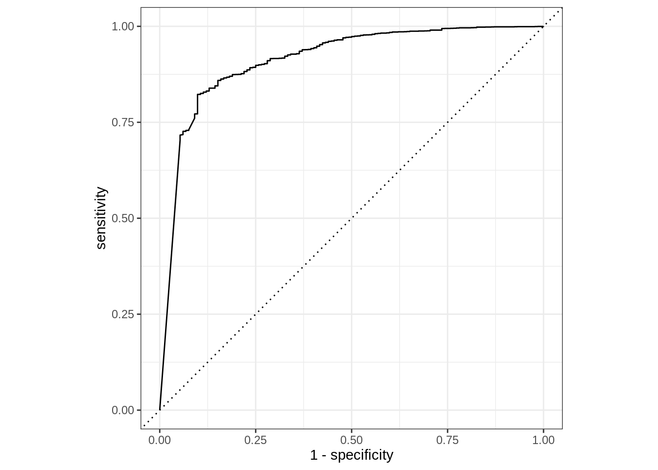
$ default   <fct> No, No, No, No, No, No, No, No, No, No, No, No, No, No, No, …

Now that everything is in one tibble, it is easy to calculate various evaluation metrics, e.g., the area under the ROC curve, using the roc_auc() function. Below is an example showing the AUROC of the model’s predictions for customers who do not default.

Default_probs |>
  roc_auc(truth = default, .pred_No)

We could also visualize the ROC via roc_curve(). The curve methods include an autoplot() function that easily creates a ggplot2 visualization.

Default_probs |>
  roc_curve(default, .pred_No) |>
  autoplot()

Based on the prediction tibble obtained, we can calculate curve methods including pr_curve, roc_curve, lift_curve, and gain_curve. In this case we are using pr_curve(), precision-recall curve. Again, because of the consistency of the interface, only the function name needs to be modified; even the argument values remain the same.

Default_probs |>
  pr_curve(default, .pred_No) |>
  glimpse()

Rows: 815
Columns: 3
$ .threshold <dbl> Inf, 1.0000000, 0.9996000, 0.9995000, 0.9993333, 0.9993333,…
$ recall     <dbl> 0.0000000, 0.7032058, 0.7088935, 0.7138056, 0.7140641, 0.71…
$ precision  <dbl> 1.0000000, 0.9974331, 0.9974536, 0.9974711, 0.9974720, 0.99…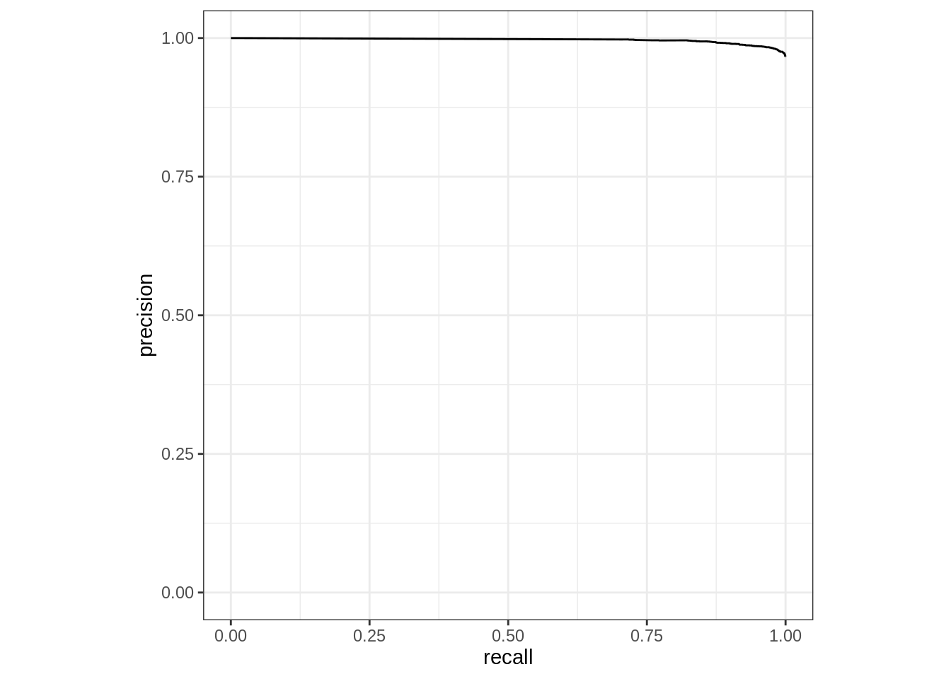

Default_probs |>
  pr_curve(default, .pred_No) |>
  autoplot()

To measured the combined single predicted value and the probability of each possible value, combine the two prediction modes (with and without prob type). In this example, using dplyr’s select() function makes the resulting tibble easier to read.

predict(Default_rf, Default_testing, type = "prob") |>
  bind_cols(predict(Default_rf, Default_testing)) |>
  bind_cols(dplyr::select(Default_testing, default))

Pipe the resulting table into metrics(). In this case, specify .pred_class as the estimate.

predict(Default_rf, Default_testing, type = "prob") |>
  bind_cols(predict(Default_rf, Default_testing)) |>
  bind_cols(dplyr::select(Default_testing, default)) |>
  metrics(default, .pred_No, estimate = .pred_class)

Exercise E

Based on the logistic regression and KNN model you built in Exercise D, make predictions for admit on the test data.

Obtain the confusion matrix from comparing with the test data.

Instead of making predictions for admit directly, make predictions for the probabilities and store the probabilities in a tibble together with the test data.